Assignment Problem and Hungarian Method: Formulation with a Complete Worked Example

Choosing the cheapest cell in an assignment table can block a better one-to-one allocation. Learners often perform row reduction but lose the logic linking the first zeros, line cover, and final assignment. A complete solution starts with the binary formulation, then follows a 4 by 4 minimisation matrix through the uncovered-value adjustment. The GATE CS exam preparation courses and test series place this method inside the wider mathematics syllabus.

What an assignment problem models, and when the model fits

In a balanced assignment problem, n workers fill n jobs. Every worker receives one job, every job goes to one worker, and c_ij is the cost of assigning Wi to Jj. The objective is to minimise total cost, not each row separately.

The Hungarian method fits one-to-one allocations with additive cell costs and a matrix made square by balancing. Unlike a transportation problem, which can send quantities greater than one, an assignment problem has unit supply and demand. Optimization in Discrete Math: LP and Worked Examples explains the wider LP, integer, assignment, transportation, and network landscape through a compact 3 by 3 assignment. The 4 by 4 matrix below isolates the Hungarian method, including binary constraints, a zero cover that forces adjustment, and extensions for maximisation and balancing.

Greedy selection fails even with two workers. For W1 = [1,2] and W2 = [2,100], taking W1-J1 = 1 forces W2-J2 = 100, totalling 101. The alternative W1-J2 = 2 and W2-J1 = 2 costs 4; the global optimum matters.

Formulate the 4 by 4 cost matrix as a binary optimisation problem

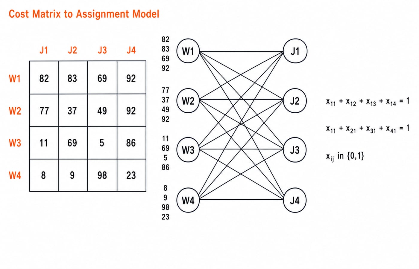
Start with this original cost matrix:

Define x_ij = 1 when Wi is assigned to Jj, and x_ij = 0 otherwise. The complete objective is:

min Z = 82x_11 + 83x_12 + 69x_13 + 92x_14 + 77x_21 + 37x_22 + 49x_23 + 92x_24 + 11x_31 + 69x_32 + 5x_33 + 86x_34 + 8x_41 + 9x_42 + 98x_43 + 23x_44.

For each worker i, impose sum_j x_ij = 1; for each job j, impose sum_i x_ij = 1; and require x_ij to be binary. A feasible solution selects four cells with no shared row or column. The matrix method avoids checking all 4! = 24 permutations.

Hungarian method reductions: create zeros without changing the best assignment

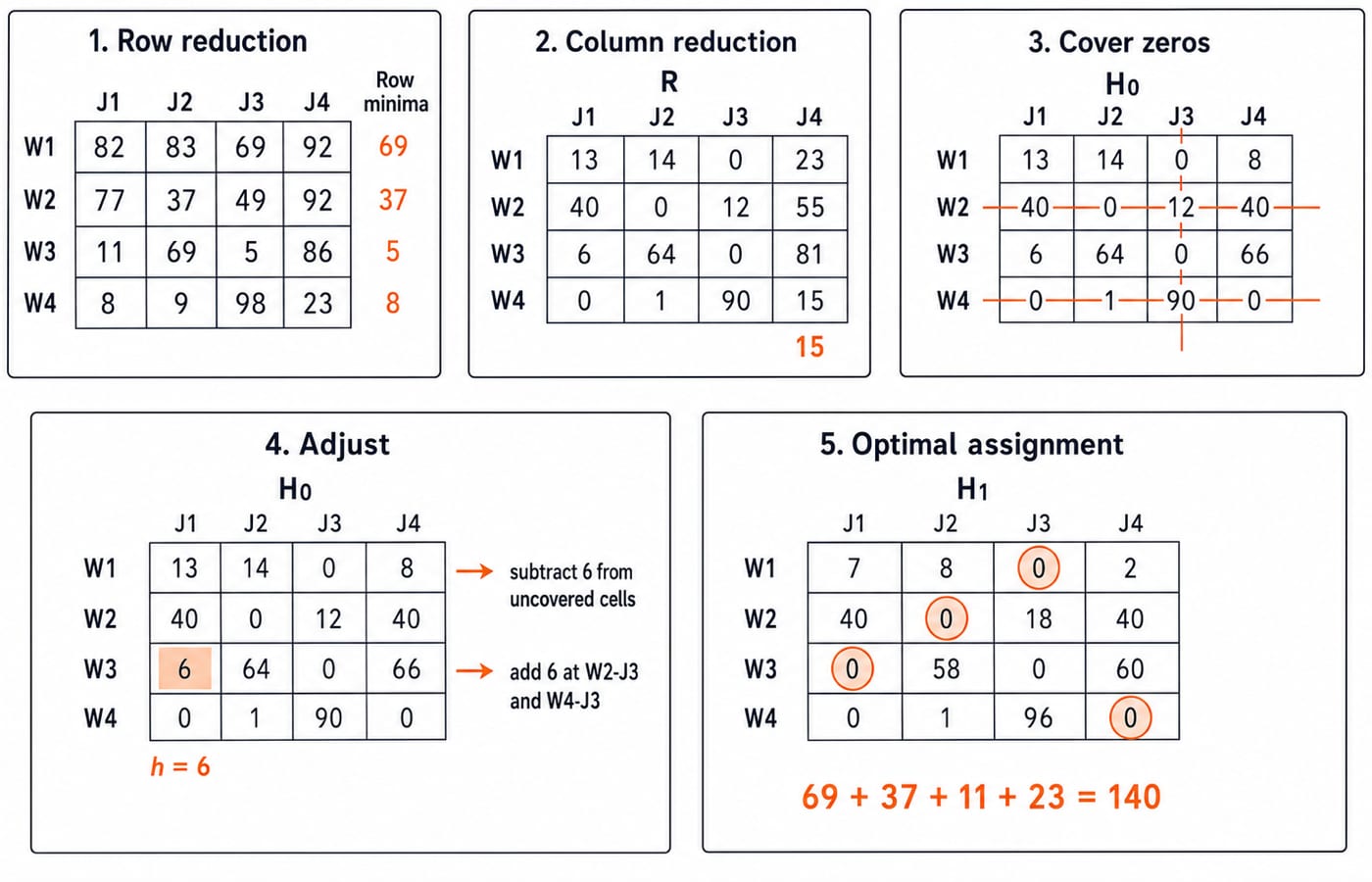
Subtracting a constant from every cell in a row preserves the best assignment: every feasible assignment uses one cell from that row, so all totals fall equally. The same applies to a column. Reduced values change, but the optimal mapping does not.

The original row minima are 69, 37, 5, 8, summing to 119. Subtracting each from its row gives the row-reduced cost matrix:

R = [[13,14,0,23], [40,0,12,55], [6,64,0,81], [0,1,90,15]].

The column minima in R are J1 = 0, J2 = 0, J3 = 0, and J4 = 15. After subtracting them, the fully reduced cost matrix is:

H0 = [[13,14,0,8], [40,0,12,40], [6,64,0,66], [0,1,90,0]].

The reduction tally 119 + 15 = 134 is a lower bound, not the answer. The zeros are (W1,J3), (W2,J2), (W3,J3), (W4,J1), and (W4,J4).

Cover the zeros, find the smallest uncovered value, and adjust

The zeros in H0 cannot supply four independent choices because W1 and W3 have their only zero in J3. Cover every zero with three minimum lines: rows W2 and W4, and column J3. Three lines are fewer than matrix order four, so adjust again.

The uncovered cells lie in rows W1,W3 and columns J1,J2,J4. Their reduced costs are 13,14,8,6,64,66, so the smallest uncovered value is h = 6 at (W3,J1).

Subtract 6 from each uncovered cell, add 6 only at the two-line intersections (W2,J3) and (W4,J3), and leave single-covered cells unchanged. The adjusted reduced cost matrix is:

H1 = [[7,8,0,2], [40,0,18,40], [0,58,0,60], [0,1,96,0]].

The adjustment raises the lower bound from 134 to 140 and creates the zero at (W3,J1), enabling four independent selections.

Read the optimal assignment and verify it in the original matrix

Select these independent zeros from H1: W1-J3, W2-J2, W3-J1, and W4-J4. Each row and each chosen column (J3,J2,J1,J4) appears once. Other zeros are not automatically assignments.

H1 also has zeros at (W3,J3) and (W4,J1), but they conflict with occupied columns after selecting W1-J3 and W3-J1. Independence, not the number of zeros, decides the mapping.

Now price the selection in the original cost matrix: W1-J3 = 69, W2-J2 = 37, W3-J1 = 11, and W4-J4 = 23. Therefore Z = 69 + 37 + 11 + 23 = 140, not zero.

The reductions and adjustment established a lower bound of 140. This feasible assignment reaches it, proving optimality: W1-J3, W2-J2, W3-J1, W4-J4, with total cost 140.

Maximisation, unbalanced matrices, forbidden cells and method boundaries

For maximisation, convert profits into costs. Given the original profit matrix P = [[62,75,80],[70,65,78],[68,72,74]], take its largest profit M = 80. The transformed cost matrix is C' = M - P = [[18,5,0],[10,15,2],[12,8,6]]. Minimising C' selects W1-J3, W2-J1, W3-J2. Its transformed cost is 0 + 10 + 8 = 18, while the original profit is 80 + 70 + 72 = 222. The check 3 x 80 - 18 = 222 works because every feasible assignment contains three cells, so the transform reverses the objective without changing feasibility.

For an unbalanced original cost matrix [[4,7,6,8],[5,3,7,6],[8,5,4,7]], add a dummy worker row [0,0,0,0]. Its assigned job is unfilled. If that has a stated penalty, use it in the dummy row instead of zero.

A forbidden pair must remain unavailable. Use a large penalty only when its scale is explained. Ties can produce several optimal mappings, and each must be checked against the original matrix. Assignment problems are not minimum spanning tree problems: Kruskal and Prim choose graph edges under a tree constraint, while Hungarian chooses one matrix cell per row and column.

Common Hungarian-method traps and representative exam-style tasks

Typical exam prompts ask you to write the binary constraints, reduce a matrix, identify a minimum zero cover, compute h, perform one adjustment, recover the original objective, convert maximisation, or balance a rectangular table. For mixed practice after the method, use Discrete Mathematics MCQs.

Assignment problem short version and the next useful step

Define binary variables and one-to-one constraints. Row-reduce, column-reduce, test for n independent zeros, cover all zeros with minimum lines, and adjust by the smallest uncovered value when needed. Select independent zeros and price them in the original matrix. The output is a feasible mapping, not a reduced matrix. Here it is W1-J3, W2-J2, W3-J1, W4-J4, costing 140.

Now reproduce H0, the three cover lines, and h = 6 without looking back. Use Engineering Mathematics for GATE Exam for a broader mathematics foundation, then GATE Guidance by Sanchit Sir for a structured preparation route.