

Linear Programming Problem Structure and Mathematical Model: A Step-by-Step Worked Example
Learn how to turn a word problem into an LP model, check feasibility, find every corner point, and identify the optimum in one consistent numerical example.
KnowledgeGate Team
Exam prep & CS education
Updated 14 Nov 20265 min read
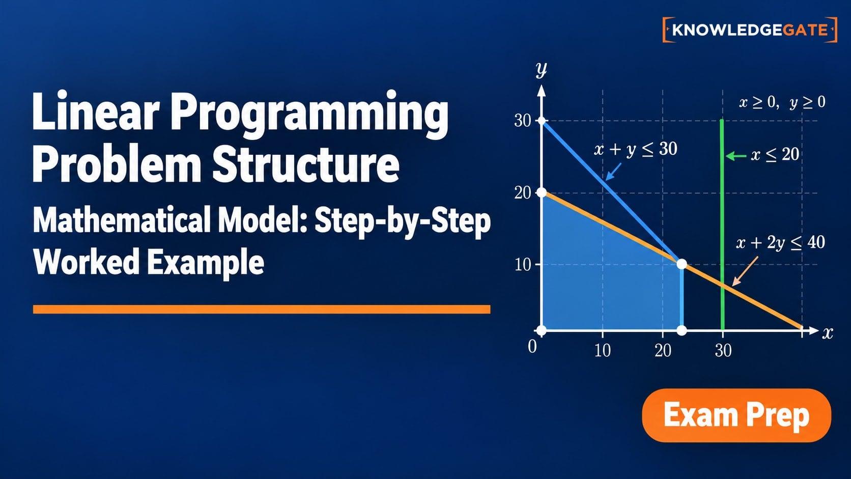
Many learners can solve two inequalities after someone has written them down, but get stuck when the information arrives as a paragraph. The real skill is converting choices, benefits and limits into one consistent mathematical model. A resource table becomes equations only when each column represents an activity and each row represents one resource; feasibility then filters the corner points before objective values identify the optimum.
What makes a problem a linear programming problem?
Linear programming, or LP, means choosing values of decision variables to maximise or minimise a linear objective while satisfying linear constraints. Here, "programming" means planning or optimisation. It does not mean writing computer code.
A quick linearity check is to inspect how every variable appears. Each variable must be raised only to the first power and multiplied by a constant. Expressions such as 30x + 20y, 2x + y <= 10 and x - y = 3 are linear. Terms such as xy, x^2, 1/x and max(x, y) are not linear in their written form.
An LP assumes proportionality, additivity, divisibility and certainty. Effects scale with activity, total effects can be added, fractions are allowed, and coefficients are known. Whole-number choices instead require an integer programming model.
The four parts of an LP model
Build an LP in this order:
Decision variables: What can change? Define every choice and its unit.
Objective function: What is being maximised or minimised?
Constraints: What resources, requirements or rules limit the choices?
Sign or domain restrictions: Which values are allowed?
The compact form is max/min Z = c^T x, subject to Ax <= b and x >= 0. Here, x holds the decisions, c holds their per-unit objective coefficients, each row of A records resource use, and b holds the limits. A constraint may instead use >= or = when required.
Optimization in Discrete Mathematics owns the wider comparison of continuous LP, integer methods, assignment, transportation and network models. Basic Terminologies in Linear Programming owns standard-form algebra, bases, BFS points and degeneracy. The four-part formulation here stays narrower: turn one resource paragraph into a consistent LP before choosing a solver method.
How to translate a word problem into equations
Define each variable with a unit. Write one objective coefficient per variable, convert each limited resource into a constraint, add non-negativity, then check units.
The wording usually reveals the inequality direction:
"At most" and "cannot exceed" mean
<=."At least" means
>=."Exactly" means
=.
Read coefficients column-wise by activity, but write constraints row-wise by resource. The two sides must use the same unit, such as capacity used and capacity available. For guided practice around the supporting concepts, use the Engineering Mathematics course.
Worked example: build the mathematical model from a resource table
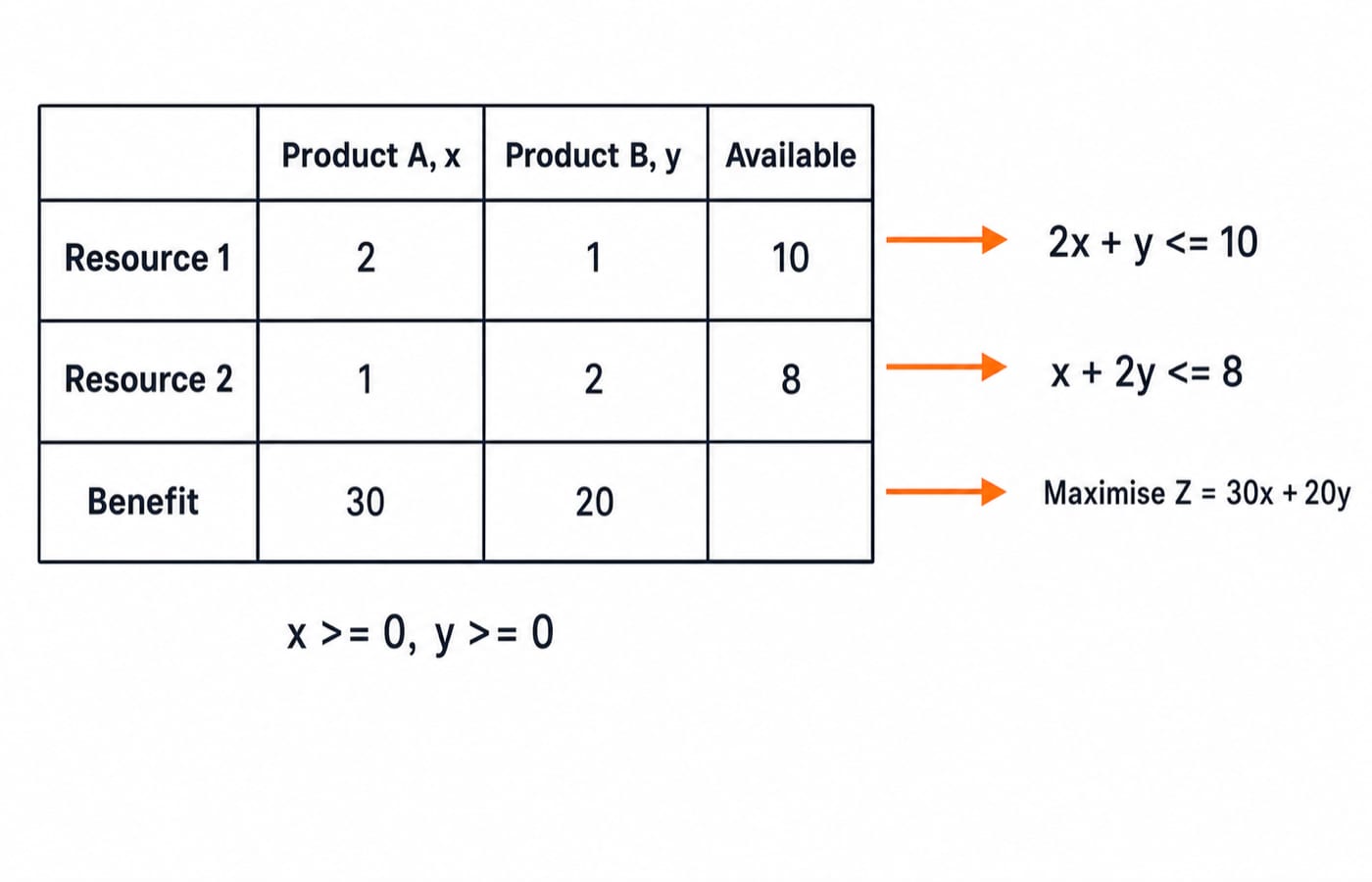
A unit schedules standard production runs of Product A and Product B. Let x be the number of A runs and y the number of B runs.
Item | Product A, | Product B, | Available |
|---|---|---|---|
Resource 1 | 2 | 1 | 10 |
Resource 2 | 1 | 2 | 8 |
Benefit per run | 30 | 20 | Not applicable |
Each run creates benefit, so the objective is to maximise:
Z = 30x + 20y
Resource 1 use is 2 units per A run and 1 per B run. With only 10 units available:
2x + y <= 10
Resource 2 use is 1 unit per A run and 2 per B run. Its capacity is 8:
x + 2y <= 8
Also require x >= 0 and y >= 0. These conditions restrict the decision domain, not resource capacity. Both inequalities point left because use cannot exceed availability.
Audit the point (3, 2). Resource 1 use is 2(3) + 2 = 8 <= 10. Resource 2 use is 3 + 2(2) = 7 <= 8. Its benefit is Z = 30(3) + 20(2) = 90 + 40 = 130. The plan is feasible, but that fact alone does not prove it is optimal.
Solve the model by the corner-point method
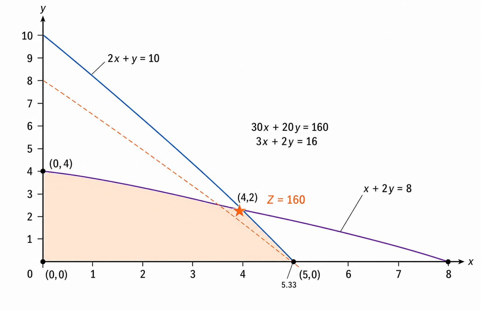
Find the boundary intercepts. For 2x + y = 10, they are (5, 0) and (0, 10). For x + 2y = 8, they are (8, 0) and (0, 4). Applying both inequalities and non-negativity leaves (0, 0), (5, 0), (4, 2) and (0, 4) as feasible vertices.
Find the non-axis intersection step by step:
2x + y = 10
x + 2y = 8
From the first equation, y = 10 - 2x. Substitute this into the second:
x + 2(10 - 2x) = 8
x + 20 - 4x = 8
-3x = -12, so x = 4 and y = 10 - 2(4) = 2.
Now evaluate every feasible corner:
Vertex | Objective calculation |
|
|---|---|---|
|
| 0 |
|
| 150 |
|
| 160 |
|
| 80 |
The optimum is (4, 2), with maximum benefit Z = 160. Checking only the axis intercepts would incorrectly stop at 150 and miss the intersection. Graphical Method in Linear Programming owns half-plane shading, objective-line movement and special geometric outcomes; this corner calculation is only the verification step for the model formulated above.
Common modelling traps and how to correct them
Treating "at least" as <= reverses the requirement. Omitting x, y >= 0 admits invalid choices. Putting capacities into the objective confuses limits with benefits, while mixed units make a constraint meaningless. Correct each error by rereading the noun and unit attached to every number.
An intersection is not automatically feasible, so test every constraint. Two intercepts are not all the corners, so list the complete feasible polygon. Do not round a fractional LP answer unless indivisibility is stated and integer restrictions are added.
For classification, xy <= 10 is nonlinear because two variables are multiplied. By contrast, 2x + y <= 10 remains linear even though it contains two variables.
How exam questions test LP problem structure
Common question shapes ask you to formulate a model from prose, test a point for feasibility, identify redundant or binding constraints, or choose the optimum from corner values. Each task checks whether variables, units, inequality directions and objective values remain consistent from the wording to the final decision.
Use this quick checklist: define variables and units, circle optimisation words, underline limits, choose inequality directions, add domain restrictions, and inspect for nonlinear terms. At (4, 2), both constraints are binding because 2(4) + 2 = 10 and 4 + 2(2) = 8.
For the surrounding syllabus and preparation routes, use the GATE CS Exam Preparation Courses & Test Series category.
The short version and what to practise next
Variables describe the choices.
The objective describes the goal.
Constraints describe the limits.
Non-negativity describes the allowed domain.
For a two-variable graphical LP, comparing all feasible corners identifies the optimum.
Rebuild this model once with capacities changed from (10, 8) to (12, 9). Derive the new constraints and corners before looking for any solution. Then compare your result with the original model and explain which constraints bind at the new optimum.
Go deeper with the full courseEngineering Mathematics for GATE Exam
Keep learning

Basic Terminologies in Linear Programming: Feasible Solutions, BFS and an Optimal Solution Worked Step by Step
Separate feasible, basic feasible and optimal solutions through geometry, slack variables, vertex enumeration and concise counterexamples.
Updated 25 Sep 20265 min read82 viewsEngineering Mathematics
Linear Equations for Aptitude: One-Variable, Two-Variable and Word-Problem Methods
Learn a reliable method for one-variable equations, two-variable systems and word problems, then check every answer against the original condition.
Updated 12 Sep 20266 min read59 viewsAptitude & Reasoning

Graphical Method in Linear Programming: Feasible Region, Corner Points and Optimality with a Worked Example
Learn the two-variable graphical method in the right order, then solve and audit a complete maximisation model without trusting the sketch alone.
Updated 21 Oct 20265 min read73 viewsEngineering Mathematics

Optimization in Discrete Mathematics: Linear Programming, Integer Methods and Worked Examples
Learn how to model and solve continuous and discrete optimization problems through a workshop LP, an integer branch-and-bound tree, an assignment matrix, and a dual.
Updated 30 Oct 20267 min readEngineering Mathematics