Spline Representation in Computer Graphics: Bezier, Hermite and B-Splines Worked Out

A spline is not merely a smooth line drawn through several dots. It is a piecewise parametric curve whose basis functions decide how stored control data influences its shape, and each representation stores that data differently. That distinction is what makes the formulas useful. One cubic curve, with controls (0,0), (2,4), (4,4) and (6,0), can be written in Hermite, Bezier and B-spline form, and its midpoint, its endpoint tangents and the continuity of its join with a neighbouring segment all follow from short hand calculations.

A spline is a piecewise parametric curve with controlled continuity

A parametric curve is written as C(u) = (x(u), y(u)) in two dimensions or C(u) = (x(u), y(u), z(u)) in three. Each segment has its own parameter interval. A cubic segment uses degree-three basis functions, while a spline can join several polynomial segments.

A useful common form is C(u) = sum N_i(u)P_i. The stored points or geometric data are P_i, and the basis functions N_i(u) provide their weights. In interpolation, the curve must pass through specified data points. In approximation, inner control points guide the shape but need not lie on the curve.

At a join, C0 continuity means equal positions. C1 also requires equal first derivatives, and C2 additionally requires equal second derivatives. G1 is weaker than C1: its tangent directions must be consistently oriented and collinear, but their magnitudes need not match. C1 requires matching derivative vectors under the chosen parameterisation.

Hermite, Bezier and B-spline forms store different control information

A cubic Hermite curve stores endpoints H0, H1 and endpoint tangents T0, T1. For 0 <= u <= 1,

C(u) = (2u^3 - 3u^2 + 1)H0 + (u^3 - 2u^2 + u)T0 + (-2u^3 + 3u^2)H1 + (u^3 - u^2)T1.

A cubic Bezier curve stores four control points:

C(u) = (1-u)^3 P0 + 3u(1-u)^2 P1 + 3u^2(1-u)P2 + u^3 P3.

It satisfies C(0)=P0, C(1)=P3, C'(0)=3(P1-P0) and C'(1)=3(P3-P2). The same Hermite curve becomes Bezier when P0=H0, P1=H0+T0/3, P2=H1-T1/3 and P3=H1.

A B-spline is specified by its degree p, control points and a nondecreasing knot vector. Its knots govern segment boundaries and continuity. With degree 3, four control points and the clamped vector [0,0,0,0,1,1,1,1], it is exactly one cubic Bezier segment. These are related ways of representing curves, not unrelated formula lists.

Worked example: evaluate a cubic Bezier point and tangent

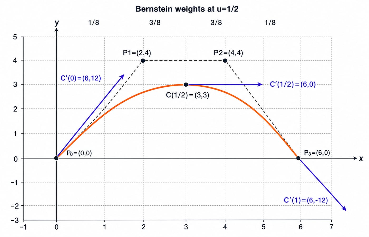
Take P0=(0,0), P1=(2,4), P2=(4,4) and P3=(6,0). At u=1/2, the four Bernstein weights are 1/8, 3/8, 3/8 and 1/8. Therefore,

C(1/2) = (1/8)(0,0) + (3/8)(2,4) + (3/8)(4,4) + (1/8)(6,0)

= (0,0) + (3/4,3/2) + (3/2,3/2) + (3/4,0) = (3,3).

Differentiate the curve:

C'(u)=3[(1-u)^2(P1-P0) + 2u(1-u)(P2-P1) + u^2(P3-P2)].

The three differences are (2,4), (2,0) and (2,-4). At u=1/2,

C'(1/2)=3[(1/4)(2,4) + (1/2)(2,0) + (1/4)(2,-4)] = 3(2,0) = (6,0).

So (3,3) is the parameter midpoint, not necessarily half the arc length, and the tangent there is horizontal. At the endpoints, C'(0)=(6,12) and C'(1)=(6,-12). Moving P1 changes the starting tangent and the segment's shape, but the endpoints remain P0 and P3.

Those endpoint values are also the Hermite data for this curve: H0=(0,0), H1=(6,0), T0=(6,12) and T1=(6,-12). The conversion rule from the previous section returns the same control polygon, since H0+T0/3=(0,0)+(2,4)=(2,4)=P1 and H1-T1/3=(6,0)-(2,-4)=(4,4)=P2. One curve, two stored descriptions.

De Casteljau subdivision reproduces the same worked point

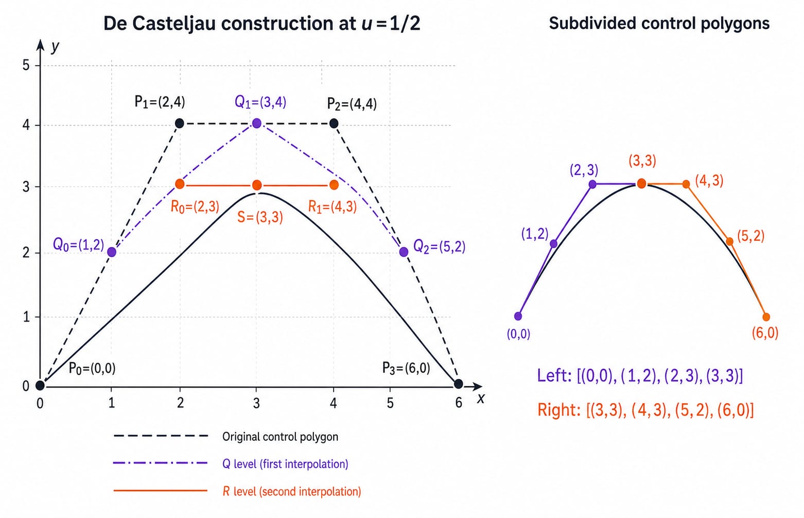
De Casteljau's construction repeatedly interpolates between neighbouring controls. At u=1/2, its first level is Q0=(1,2), Q1=(3,4) and Q2=(5,2). The second level is R0=(2,3) and R1=(4,3). The final point is S=(R0+R1)/2=(3,3), matching the Bernstein calculation.

The left subdivided control polygon is [(0,0),(1,2),(2,3),(3,3)]. The right one is [(3,3),(4,3),(5,2),(6,0)]. These describe two parameter intervals of the same geometric curve. Since every constructed point is an affine combination of the controls, the curve stays inside their convex hull and follows the controls under an affine transformation.

Joining cubic segments: position, tangent and curvature conditions

Call the worked curve A, with controls A0=(0,0), A1=(2,4), A2=(4,4), A3=(6,0). Add curve B with B0=(6,0), B1=(8,-4), B2=(10,-4), B3=(12,0). The join is C0 because A3=B0=(6,0).

For first derivatives,

A'(1)=3(A3-A2)=3(2,-4)=(6,-12)

B'(0)=3(B1-B0)=3(2,-4)=(6,-12).

The derivative vectors match, so the join is C1. Now check curvature-related second derivatives:

A''(1)=6(A3-2A2+A1)=6(0,-4)=(0,-24)

B''(0)=6(B2-2B1+B0)=6(0,4)=(0,24).

They differ, so this join is not C2. For equally parameterised cubic Bezier segments, set B0=A3 for C0 and B1=2A3-A2 for C1. Test the second-control-point relation separately before claiming C2. Collinear handles alone establish only a geometric tangent condition unless scaling and parameterisation also match.

B-splines add local control through knots and basis support

Moving a Bezier control point can affect its whole segment. A degree-p B-spline control point P_i acts only where its basis N_{i,p}(u) is nonzero, over [u_i,u_{i+p+1}). This local support lets us edit a long composite curve without disturbing every earlier span.

At an internal knot of multiplicity r, a degree-p B-spline is generally C^(p-r) continuous. For a cubic, a simple internal knot gives C2, a double knot gives C1, and a triple knot gives C0. Repeating a clamped endpoint p+1=4 times makes the curve reach its endpoint control point. The worked curve is itself such a B-spline: degree 3, controls P0 to P3 and knot vector [0,0,0,0,1,1,1,1] reproduce the same segment from (0,0) to (6,0).

No representation is universally best. The right choice depends on whether endpoint derivatives, simple segment controls or local multi-segment editing matter most.

Traps and the question shapes that expose them

Do not assume that a curve passes through every control point. A Bezier segment interpolates its endpoints, while inner controls influence its shape. Also, do not treat u as distance travelled: C(1/2)=(3,3) is only a parameter midpoint unless the curve uses arc-length parameterisation.

A visually smooth join is not automatically C1 or C2; compare derivatives. The two-segment join above is C1 but not C2. For B-splines, write the degree, control count and complete knot vector before applying a rule, because degree and control-point count are not interchangeable.

Common question shapes ask you to evaluate a point or tangent, identify a curve property, or derive a join condition. As a quick check, at u=1/4 the weights are 27/64, 27/64, 9/64 and 1/64. Substitution gives C(1/4)=(1.5,2.25).

Spline representation sits in the computer graphics unit of the UGC NET Computer Science syllabus. UGC NET Computer Science syllabus areas maps where graphics falls in Paper 2, and UGC NET Computer Science high-yield topics ranks the units worth revising first; the official syllabus text and paper instructions are published on the NTA portal.

The short version and the next useful step

A spline joins polynomial pieces, and basis functions blend its stored control data. Continuity must be checked at every join, while knots give B-splines local control. For the cubic curve, C(1/2)=(3,3) and C'(1/2)=(6,0). Keep that calculation beside the definitions so the notation remains concrete.

Now replace P1=(2,4) with P1=(2,2), keeping P0=(0,0), P2=(4,4) and P3=(6,0). Verify at u=1/2 that the new point is (3,2.25) and the derivative is (6,1.5), then explain why the curve moves while both endpoints stay fixed.

For a structured subject path, continue with NTA-UGC-NET Paper 2. For timed practice, use the UGC NET Computer Science and Applications Test Series.