

Introduction and Types of Data MCQs: 11 Questions with Worked Solutions
Separate counts from measurements, read histograms, calculate grouped means and test distribution, trend and price-index rules with worked questions.
KnowledgeGate Team
Exam prep & CS education
Updated 31 Oct 20267 min read

Knowing the word “data” does not always help you distinguish counts from measurements or interpret grouped displays correctly. These questions separate data types, histograms, grouped means, distributions, trends and index numbers. Attempt each question before reading its solution, and write down the rule you used so that a lucky guess does not hide a misunderstanding.
1. Recognise the discipline and the data type
Before choosing a formula, ask whether you are counting objects, measuring a quantity or recording a category.
Q1. Identify the discipline
The science which deals with the methods of collecting, classifying, presenting, comparing and interpreting numerical data is called
(a) statistics
(b) mathematics
(c) geometry
(d) probability
Answer: (a), statistics. The five operations describe statistical work: collecting, classifying, presenting, comparing and interpreting observations.
For example, collect scores 40, 50, 60, arrange them in ascending order and calculate their mean: (40 + 50 + 60)/3 = 150/3 = 50. This summarises the observed scores. It is a descriptive summary, not a prediction of the next student's score.
Q2. Separate measurements from counts
Among the following, identify the continuous type of data :
(a) Number of languages a person speaks
(b) Number of children in a household
(c) Population of cities
(d) Weight of students in a class
Answer: (d), Weight of students in a class. Languages, children and people are counted in whole numbers, so these variables are discrete. Weight is measured: 52.4 kg and 52.45 kg are possible even if a scale rounds its display.
For a qualitative contrast, blood groups A, B and O are category labels, not counts or measurements.
2. Read histogram bars with the right assumptions
First identify what the horizontal axis represents. Continuous class intervals and named categories require different readings.
Q3. Identify the grouped display
The graphical representation of a grouped continuous frequency distribution using adjoining class intervals is called:
(a) Bar chart
(b) Line chart
(c) Histogram
(d) Pie chart
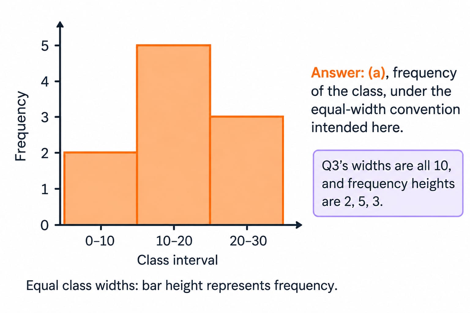
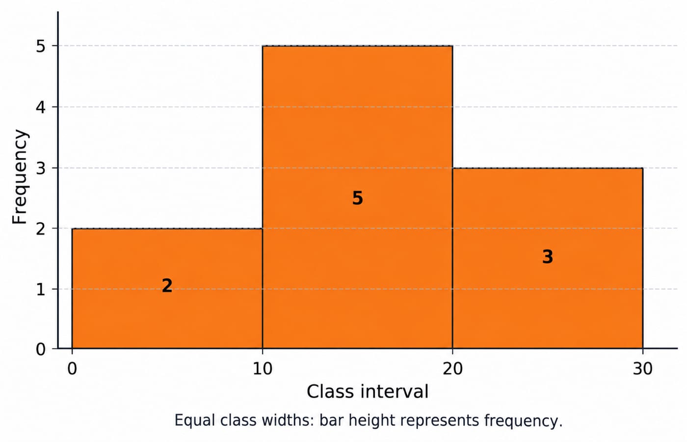
Answer: (c), Histogram. Its rectangles adjoin because they represent adjoining intervals of a continuous variable. Take equal-width intervals 0-10, 10-20, 20-30 with frequencies 2, 5, 3. Their touching bars show how observations are distributed across those intervals.
By comparison, a bar chart separates categories, a line chart connects points such as successive time observations, and a pie chart uses sectors for parts of a whole.
For more practice on the ideas in Q2 and Q3, work through this Statistics module for related practice.
Q4. Interpret bar height carefully
The height of a rectangle in a histogram shows:
(a) frequency of the class
(b) width of the class
(c) upper limit of the class
(d) lower limit of the class
Answer: (a), frequency of the class, under the equal-width convention intended here. Q3's widths are all 10, and frequency heights are 2, 5, 3.
For unequal widths, use frequency density so that area represents frequency. Widths 10 and 20 with frequencies 5 and 10 give heights 5/10 = 0.5 and 10/20 = 0.5.
Revisit the histogram-height solved explanation, then compare categorical displays in Bar Charts for Data Interpretation: Solved Examples.
3. Compute a grouped mean without losing the weights
Weight each class midpoint by its frequency.
Q5. Calculate the grouped mean
Calculate the mean of the following
Class interval | Frequency |
|---|---|
90 - 100 | 10 |
80 - 90 | 15 |
70 - 80 | 14 |
60 - 70 | 12 |
50 - 60 | 9 |
(a) 73.2
(b) 75.8
(c) 74.6
(d) 71.5
Answer: (b), 75.8. Midpoint = (lower limit + upper limit)/2; multiply by frequency.
Class interval | Frequency f | Midpoint m | f x m |
|---|---|---|---|
90 - 100 | 10 | 95 | 950 |
80 - 90 | 15 | 85 | 1275 |
70 - 80 | 14 | 75 | 1050 |
60 - 70 | 12 | 65 | 780 |
50 - 60 | 9 | 55 | 495 |
Total | 60 | 4550 |
sum f = 10+15+14+12+9 = 60; sum fm = 950+1275+1050+780+495 = 4550.
Grouped mean = 4550/60 = 75.8333…, rounded to 75.8. Midpoints approximate unknown individual observations. For the first row, (90 + 100)/2 = 95 and 10 x 95 = 950. Repeat this operation for every row; keep the frequency attached to its own class. The unweighted midpoint average, 375/5 = 75, ignores unequal frequencies. Revisit the grouped-mean worked solution.
4. Distinguish skewness, normal spread and binomial outcomes
After calculating averages, examine distribution shapes, measure spread around the mean and count successes in repeated trials.
Q6. Find the direction of skewness
When most of the students obtain high scores, the distribution is termed as:
(a) Normal
(b) Positively skewed
(c) Negatively skewed
(d) Leptokurtic
Answer: (c), Negatively skewed. The intended pattern has most scores towards the high end and a tail stretching towards low scores, or leftwards. Name the skew from the tail, not the crowded side.
For illustration, scores 20, 80, 85, 90, 90, 95, 100 sum to 560. Their mean is 560/7 = 80; their median is the fourth value, 90. The low score pulls the mean below the median. Leptokurtic concerns kurtosis, especially tail heaviness, rather than left-right direction.
Q7. Apply the normal-model rule
In a normal distribution, what percentage of the data lies within one Standard deviation from the Mean ?
(a) 68%
(b) 95%
(c) 99.7%
(d) 50%
Answer: (a), 68%, approximately. With mean 50 and standard deviation 5, one standard deviation on either side gives 50 - 5 = 45 to 50 + 5 = 55.
About 68% lies within [45, 55]. Two standard deviations give [40, 60], containing about 95%; three give [35, 65], containing about 99.7%. These percentages describe a normal model, not every dataset. “Within” includes both sides, not just half the symmetric curve.
Q8. Identify a binomial trial
Which of the following is a characteristic of a binomial distribution ?
(a) The events are dependent
(b) The outcomes are continuous
(c) There are two outcomes, success or failure
(d) The Mean is equal to the Mode
Answer: (c), There are two outcomes, success or failure. This describes each trial. The binomial variable counts successes over a fixed number n of independent trials with constant success probability p.
For three fair tosses, let heads be success: n = 3, p = 0.5, and X can be 0, 1, 2 or 3. Exactly two heads occur as HHT, HTH or THH. Thus P(X = 2) = 3 x (0.5)^2 x 0.5 = 3/8. Two outcomes alone do not establish all binomial assumptions.
5. Shift a trend origin and explain moving-average endpoints
Track the time variable and where each average belongs.
Q9. Change the trend origin
The trend line with 1975 as origin is Y=20.6+1.68X, the trend line with 1971 as origin will be -
(a) Y = 20.6 + 6.72X
(b) Y = 13.88 + 1.68X
(c) Y = 34.61 + 1.68X
(d) Y = 26.32 + 6.72X
Answer: (b), Y = 13.88 + 1.68X. Let t denote the year. Then X_old = t - 1975 and X_new = t - 1971, giving X_old = X_new - 4.
Substitute: Y = 20.6 + 1.68(X_new - 4) = 20.6 - 6.72 + 1.68X_new = 13.88 + 1.68X_new.
Check at t = 1975: X_new = 4, so Y = 13.88 + 6.72 = 20.6. Only the intercept changes; the slope remains 1.68. See the trend-origin solved example.
Q10. Understand unavailable endpoint ratios
Which of the following methods to measure seasonal variations comparatively utilizes the given data less?
(a) Simple average method
(b) Ratio to trend method
(c) Ratio-to-moving-average method
(d) Link relative method
Answer: (c), Ratio-to-moving-average method. Centred moving averages cannot be formed at certain endpoints, so those periods lack seasonal ratios.
For quarterly observations 10, 12, 14, 16, 18, 20, 22, 24, the four-term moving averages are 13, 15, 17, 19, 21. For example, (10 + 12 + 14 + 16)/4 = 13.
Centre consecutive averages: (13 + 15)/2 = 14, then 16, 18, 20, located at periods 3-6. Ratios are available at four of eight periods here. Endpoint observations still contribute to interior averages; their raw data are not wholly discarded. The loss depends on the averaging span.
6. Choose the right average for a price index
Q11. Recognise the Drobisch-Bowley formula
The Drobisch-Bowley price index formula is -
(a) Geometric mean of Laspeyres’ and Paasche’s index formula
(b) Arithmetic mean of Laspeyres’ and Paasche’s index formula
(c) Weighted mean of Laspeyres’ and Paasche’s index formula
(d) None of the above
Answer: (b), Arithmetic mean of Laspeyres’ and Paasche’s index formula. If Laspeyres’ index L = 120 and Paasche’s index P = 125, the Drobisch-Bowley index is (L + P)/2 = (120 + 125)/2 = 245/2 = 122.5.
The geometric mean is sqrt(120 x 125) = sqrt(15000) approximately 122.47, associated with Fisher's ideal index. These results are close, but the formulas differ. Identify whether the rule adds or multiplies the indices before calculating.
7. Turn each data mistake into a revision rule
Answer key: 1 (a), 2 (d), 3 (c), 4 (a, equal widths), 5 (b), 6 (c), 7 (a), 8 (c), 9 (b), 10 (c), 11 (b).
Use the answer key to label each miss as a definition, assumption or arithmetic error. A count-versus-measurement miss needs a definition check; a histogram-height miss needs an assumption check. Re-solve only the missed items the next day, showing your steps before checking the key.
For structured aptitude preparation, explore the Aptitude Course for Placement as your next study option.
If you are comparing broader preparation routes, browse the placement preparation courses and choose according to the topics you still need to practise.
Go deeper with the full courseDiscrete Mathematics
Keep learning

Factors, Multiples and Prime Factorization: 11 Questions with Worked Solutions
Confusing prime factors with total factors? Attempt these 11 questions, then check each calculation to learn divisor counting, odd and even restrictions, sums and multiples.
Updated 5 Nov 20267 min readDiscrete Mathematics MCQs

Linear Inequalities and Modulus Questions with Solutions: 11 Solved MCQs
Work through 11 linear inequalities and modulus MCQs with complete solutions. Each answer shows the case, graph feature, endpoint or algebraic step that decides it.
Updated 14 Nov 20266 min readAptitude & Reasoning

Sorting MCQs: 11 Solved Introduction to Sorting Questions with Explanations
Attempt 11 Introduction to Sorting MCQs before checking concise, teacher-led solutions on stability, in-place sorting, external sorting, complexity, and exchange counting.
Updated 27 Aug 20267 min readAlgorithms MCQs

Data Hazards in Pipelining: Types, Solutions and Worked Examples
Follow one three-instruction trace to see exactly when a load-use pair stalls and when ALU forwarding works. Then compare the same trace without forwarding.
Updated 14 Nov 20266 min readComputer Organization & Architecture