Optimization in Discrete Mathematics: Linear Programming, Integer Methods and Worked Examples

An optimization question begins as prose, but your answer depends on choosing variables, translating restrictions, and deciding whether fractions are allowed. That last decision changes the answer: ordinary linear programming permits real-valued decisions, while discrete optimization adds integer, binary, assignment, scheduling, or network structure. A workshop with 8 machine hours and 8 labour hours reaches a profit of 560/3, about 186.67, when fractions of a product are allowed, but only 180 once whole units are required. Rounding both coordinates of (8/3, 8/3) up to 3 lands outside the feasible region altogether.

Optimization vocabulary: objective, constraints and feasible solutions

A mathematical optimization model has six basic parts:

• Decision variables represent the choices.

• The objective function states what to maximise or minimise.

• Constraints state what the choices must satisfy.

• The domain declares whether variables are real, integer, or binary.

• The feasible set contains every point satisfying these rules.

• A feasible solution is one such point. An optimal solution has the best objective value.

For example, maximise z = 3x + 5y subject to x + y <= 6, x >= 0, and y >= 0. The point (2, 3) is feasible because 2 + 3 <= 6, and it gives z = 3(2) + 5(3) = 21. The point (4, 3) is infeasible because 4 + 3 > 6.

A fractional answer may suit divisible material but not people, machines, jobs, or packets. The feasible region is the intersection of the constraint sets, so intersection behaves here exactly as it does in Set Theory and Relations.

Turn a word problem into a mathematical model

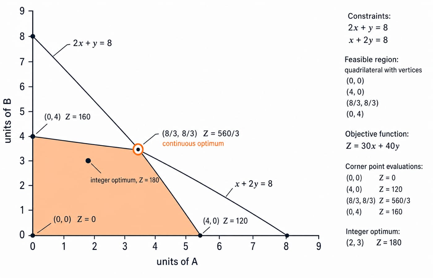
A workshop makes products A and B. One unit of A uses 2 machine hours and 1 labour hour and contributes 30 units of profit. One unit of B uses 1 machine hour and 2 labour hours and contributes 40 units of profit. The workshop has 8 machine hours and 8 labour hours.

Let x and y be the quantities of A and B. The continuous model is:

maximise Z = 30x + 40y

subject to:

• 2x + y <= 8 for machine hours

• x + 2y <= 8 for labour hours

• x >= 0, y >= 0

Each left-side coefficient is the resource consumed by one unit, each right side is the available capacity, and non-negativity is a domain condition. If products must be whole units, add x, y are non-negative integers. That line can change the answer. If symbolic translation feels unfamiliar, first practise turning statements into conditions, as in propositional and predicate logic.

Solve the continuous relaxation by the graphical method

The feasible polygon has four corners. Test all of them, not just the axis intercepts:

To find the non-axis intersection, solve 2x + y = 8 and x + 2y = 8. Subtracting the second equation from the first gives x - y = 0, so x = y. Substitution gives 3x = 8, hence x = y = 8/3. Its value, 560/3, is the continuous optimum. Checking only intercepts would incorrectly select (0, 4).

Enforce integer decisions with branch and bound

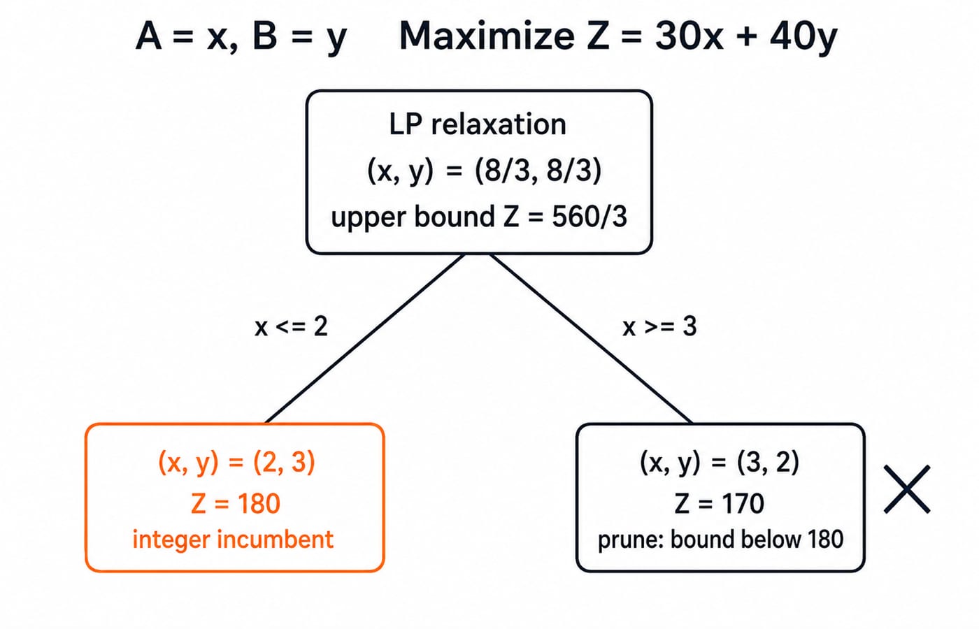
When products are indivisible, (8/3, 8/3) is not allowed. Branch on the fractional value of x.

• In the branch x <= 2, setting x = 2 leaves y <= 4 from the machine constraint and y <= 3 from the labour constraint. Thus (2, 3) is best, with Z = 30(2) + 40(3) = 180.

• In the branch x >= 3, setting x = 3 leaves y <= 2 and y <= 5/2. Thus (3, 2) is best, with Z = 30(3) + 40(2) = 170.

Therefore the integer optimum is (2, 3), not a point obtained by instinctive rounding: rounding both coordinates of (8/3, 8/3) up to 3 gives (3, 3), which needs 9 machine hours against the 8 available. The relaxation value 560/3 is an upper bound for this maximisation problem, while 180 is the best feasible integer value so far, called the incumbent. Any branch whose own bound is at most 180 can be pruned, which is what closes the x >= 3 branch: its bound is 170.

Exhaustive search checks every candidate, branch and bound uses bounds to eliminate candidates, dynamic programming reuses subproblem results, and a greedy method makes locally attractive choices. They are not interchangeable recipes.

Recognise assignment, transportation and network forms

Consider this assignment cost matrix for agents A, B, C and jobs 1, 2, 3:

Subtract each row minimum. The rows become A: [7, 0, 5], B: [3, 1, 0], and C: [4, 7, 0]. Column 1 has minimum 3, so subtract it to obtain A: [4, 0, 5], B: [0, 1, 0], and C: [1, 7, 0]. The total reduction is 2 + 3 + 1 + 3 = 9, a lower bound on every assignment.

Choose independent zeros A to 2, B to 1, and C to 3. They occupy distinct rows and columns, so this complete zero assignment reaches the lower bound and is optimal. In the original matrix its cost is 2 + 6 + 1 = 9. The next-best assignment, A to 2, B to 3, and C to 1, costs 2 + 3 + 5 = 10.

Assignment gives one job to each agent, so its variables are 0 or 1 and every row and every column is used exactly once. Transportation moves quantities from supplies to demands, so its variables are shipment amounts and the balancing condition compares total supply with total demand. PERT and CPM schedule activities under precedence restrictions. Shortest paths, spanning trees, matching, and scheduling all use graph structure, but not the same algorithm. Graph Theory for GATE CS sets out that vocabulary.

Read duality and special cases correctly

The dual of the workshop relaxation is:

minimise W = 8u + 8v

subject to 2u + v >= 30, u + 2v >= 40, and u, v >= 0. At the optimum both constraints bind. From 2u + v = 30, take v = 30 - 2u. Substitute into u + 2v = 40:

u + 2(30 - 2u) = 40, so -3u = -20 and u = 20/3.

Then v = 30 - 40/3 = 50/3. Therefore W = 8(20/3) + 8(50/3) = 560/3, matching the primal optimum. Here u and v act as marginal values for machine-hour and labour-hour capacities within this model.

Keep four special cases separate:

• Infeasible: x + y <= 2 and x + y >= 5 cannot both hold.

• Unbounded: maximise x + y subject only to x - y >= 0, x, y >= 0. Taking x = y = t allows any t >= 0.

• Multiple optima: maximise x + y subject to x + y <= 4, x, y >= 0. Every point on x + y = 4 in the first quadrant is optimal.

• Degenerate: at (2, 0), three constraints (x <= 2, x + y <= 2, y >= 0) are all active, one more than the two a vertex needs in the plane.

No feasible solution, an unbounded objective, and more than one optimum are different conclusions requiring different evidence.

How GATE-style questions and interviews test optimization

Common tasks ask you to translate prose, identify a feasible or optimal solution, take a graphical or simplex step, construct a dual, distinguish special cases, or solve a small structured instance. Interviews apply the same modelling habit to scheduling, resource allocation, shortest paths, matching, knapsack, and capacity planning.

Before naming an algorithm, ask: What are the decisions? What must be optimised? What may not be violated? Marks, question counts and the exact CS syllabus wording are published on the official GATE portal, and that is the copy to trust.

Short version and the next practice step

Revise optimization in this order:

1. Define the decision variables.

2. Write the objective.

3. Translate every constraint.

4. Declare real, integer, or binary domains.

5. Solve and check feasibility.

6. Interpret the optimum in the original words.

Next, solve one modelling question, one graphical question, and one assignment or network question. For each rejected option, identify which condition it breaks. The optimization topic on KnowledgeGate carries around 40 practice questions across linear programming basics, the graphical method, transportation, assignment and duality, and the GATE CS exam preparation courses and test series listing shows where the topic sits beside the rest of the paper.

GATE Guidance by Sanchit Sir covers the subject-wise plan for the whole paper, and the GATE Test Series gives timed sets where the modelling habit is tested under clock pressure. Keep the modelling sequence visible while you practise, because a correct algorithm cannot rescue an incorrect model.