Data Mining and Data Warehouse Explained: Concepts, OLAP and Worked Examples

A database, a data warehouse, OLAP and data mining all work with data, but they solve different problems. A system that records today's orders is not automatically a warehouse, and calculating a monthly total is analysis but not necessarily data mining. Six orders from two sources move through ETL into a star schema, where exact OLAP totals are calculated. Support, confidence and lift are calculated from five separate baskets as part of the broader CS Fundamentals material.

Data warehouse, OLAP and data mining answer different questions

An operational database captures current transactions, such as inserting an order or updating stock. A data warehouse is an integrated, historical store organised for analysis. It is subject-oriented around areas such as sales, integrated across sources, time-variant because it preserves history, and non-volatile because routine transactions do not continuously overwrite that analytical history. Controlled corrections and new loads can still occur.

OLAP provides fast, multidimensional summaries and navigation. Data mining searches for useful, non-obvious patterns or predictive structure with statistical and machine-learning methods. "January units by city" is an OLAP aggregation. Finding that diaper baskets are unusually associated with beer is a mining result. A warehouse can support reporting without mining, while mining can use data outside a warehouse. They are complementary, not synonyms or a compulsory pair. For Apriori pruning and k-means iterations, continue with Data Warehousing and Data Mining in DBMS; the ETL trace, schema grain, OLAP totals and single-rule calculation below establish the prerequisite path.

From operational sources to a data warehouse

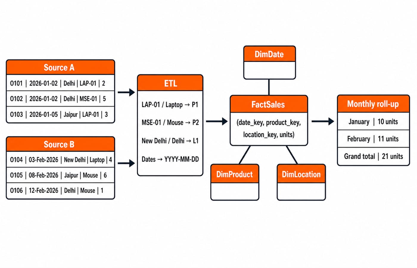
The full flow is operational sources -> staging -> ETL/ELT -> warehouse -> data marts or semantic layer -> OLAP reports and mining models. Extract collects rows, sometimes using SQL queries and joins across source tables. Transform parses 03-Feb-2026 as 2026-02-03, maps LAP-01 and Laptop to P1, and standardises New Delhi and Delhi as L1. Load places the cleaned records into analytical storage.

Staging isolates questionable rows before they enter history. Reject an order whose ID is blank, deduplicate a repeated O104, and quarantine an order with a negative unit count until its business meaning is confirmed. One extraction join alone does not create a warehouse.

Fact grain, dimensions, star and snowflake schemas

Fix the grain before naming columns. Here, each sales record represents one order line. Its measure is units; its foreign keys are date_key, product_key and location_key. The central table is FactSales(date_key, product_key, location_key, units), with DimDate, DimProduct and DimLocation providing context. Order ID can remain a degenerate dimension when analysts must trace a fact back to the source.

In a star schema, denormalised dimensions join directly to the fact. A location record can keep its location_key, city and region together. A snowflake splits a hierarchy, perhaps into DimLocation(location_key, city, region_key) and DimRegion(region_key, region). The snowflake reduces repeated hierarchy text but adds another join; the choice is workload-driven. DBMS normalization explained covers the related OLTP trade-off.

Worked warehouse example: six orders and OLAP operations

Every value below is synthetic teaching data, not a live business statistic.

The base totals are:

• January: 2 + 5 + 3 = 10; February: 4 + 6 + 1 = 11; grand total: 10 + 11 = 21.

• Delhi: 2 + 5 + 4 + 1 = 12; Jaipur: 3 + 6 = 9; city total: 12 + 9 = 21.

• Laptop: 2 + 3 + 4 = 9; Mouse: 5 + 6 + 1 = 12; product total: 9 + 12 = 21.

A roll-up turns daily rows into January 10 and February 11. A drill-down expands January 10 into Delhi 7 and Jaipur 3. A slice keeps the data for January. A dice selects multiple dimensions, such as both months for Laptop in Delhi and Jaipur; the non-zero cells are 2, 3 and 4, totalling 9. A pivot then rotates the month-city view so cities become rows and months become columns:

Pivoting changes presentation, not the underlying total.

What data mining does and where KDD fits

Mining tasks differ by output. Classification predicts a label such as whether renewal occurs. Regression predicts a number such as next month's unit demand. Clustering forms groups without provided labels. Association finds co-occurring items, while anomaly detection flags unusually different records. A chart or SQL aggregate is not automatically a model.

The wider KDD process selects relevant data, cleans it, integrates sources, transforms features, runs a mining method, evaluates whether the result is valid and useful, then presents it. Data preparation belongs to knowledge discovery even though the algorithmic mining step is narrower. Leakage can invalidate the result: a renewal classifier may use logins_last_30_days = 4, but it must not use renewal_status = no as an input when that same field is the label being predicted.

Worked data-mining example: support, confidence and lift

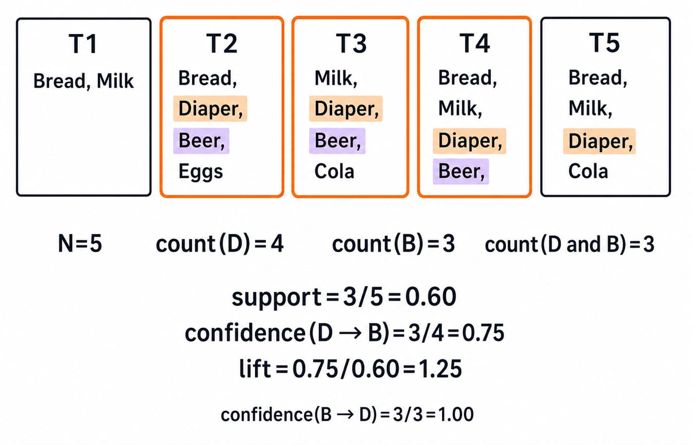
Use five baskets: T1 = {Bread, Milk}, T2 = {Bread, Diaper, Beer, Eggs}, T3 = {Milk, Diaper, Beer, Cola}, T4 = {Bread, Milk, Diaper, Beer}, and T5 = {Bread, Milk, Diaper, Cola}. Test Diaper -> Beer with minimum support 0.50 and minimum confidence 0.70.

Count first. Diaper occurs in T2, T3, T4 and T5, so count(Diaper) = 4. Beer occurs in T2, T3 and T4, so count(Beer) = 3. Both occur in T2, T3 and T4, so count(Diaper and Beer) = 3. There are N = 5 baskets.

• Support: support(Diaper and Beer) = 3/5 = 0.60.

• Confidence: confidence(Diaper -> Beer) = 3/4 = 0.75.

• Lift: 0.75 / (3/5) = 0.75 / 0.60 = 1.25.

The rule passes both thresholds. Lift above 1 indicates positive association in this tiny dataset, not causation. Direction matters: reversing the rule gives confidence(Beer -> Diaper) = 3/3 = 1.00, although support remains 0.60.

Exam traps and checks to practise

Test yourself with five quick checks:

1. History organised by time shows which property? Time-variant.

2. What is the fact grain here? One order line per row.

3. January 10 drilled down by city? Delhi 7, Jaipur 3, total 10.

4. Labels provided or absent? Classification uses labels; clustering does not.

5. confidence(Beer -> Diaper)? 3/3 = 1.00.

The short version and your next study step

• Operational databases capture current events.

• ETL standardises and loads history.

• A warehouse organises that history for analysis, totalling 21 units here.

• OLAP summarises history across dimensions.

• Data mining discovers patterns, with support 0.60, confidence 0.75 and lift 1.25 in this example.

For a broader DBMS and interview foundation, continue with Computer Science Fundamentals for Placements by Sanchit Sir. Next, redraw the six-order star schema, recompute all five OLAP operations, then reverse the basket rule and explain why confidence changes.