Data Warehousing and Data Mining in DBMS: Star Schema, OLAP Operations and Apriori with Worked Examples

You may know tables, SQL and normalization, yet warehousing feels separate because of terms such as fact table, roll-up, support and confidence. Each of those words is really an instruction to compute something: a grand total across quarters, a support fraction over five transactions, a cluster mean over four points. Work each one on a small dataset by hand and the vocabulary stops being vocabulary.

OLTP vs OLAP: why a warehouse is not just a big database

A data warehouse has four textbook properties:

• Subject-oriented: data is organised around subjects such as sales, products or customers.

• Integrated: data from different sources is cleaned into consistent names, formats and keys.

• Time-variant: historical snapshots are retained, so changes can be analysed across time.

• Non-volatile: data is loaded and read for analysis, not updated in place by day-to-day transactions.

Normalization rules the OLTP world. Warehousing deliberately accepts some redundancy, and a star schema shows why.

Star schema worked end to end

Use this central fact table:

FactSales(date_key, product_key, store_key, units_sold, revenue)

It connects to three dimensions:

• DimDate(date_key, day, month, quarter, year)

• DimProduct(product_key, product_name, category, brand)

• DimStore(store_key, city, state, region)

The fact holds measures and foreign keys; dimensions provide grouping and filtering context.

DimProduct repeats category and brand, so the star is denormalized. A snowflake could use DimProduct(product_key, product_name, brand_key) and DimBrand(brand_key, brand, category). This removes repetition but adds a join.

For “total revenue by region for quarter Q2”, join FactSales to DimStore and DimDate, filter Q2, then group by region. Warehouse queries use this join-plus-GROUP BY pattern.

SELECT s.region, SUM(f.revenue) AS revenue
FROM FactSales f
JOIN DimStore s ON f.store_key = s.store_key
JOIN DimDate d ON f.date_key = d.date_key
WHERE d.quarter = 'Q2'
GROUP BY s.region;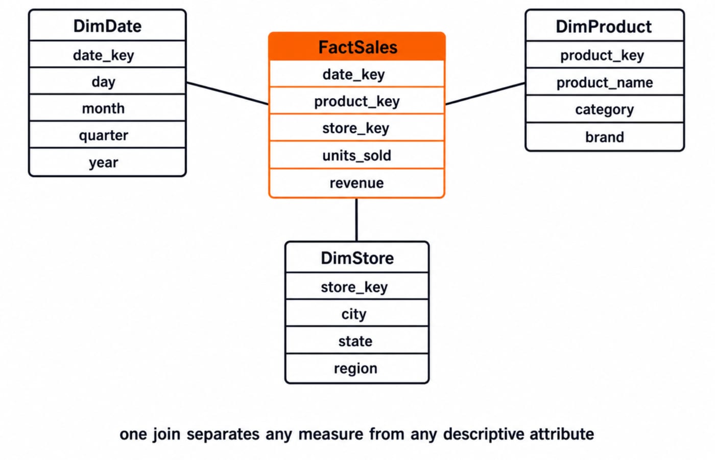

The data cube and OLAP operations on real numbers

Consider units sold across Region, Product and Quarter:

Now compute each OLAP operation:

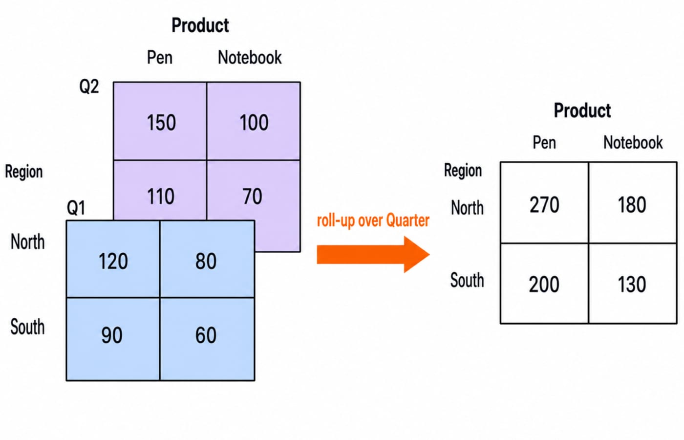
• Roll-up combines quarters into a year. North-Pen is 120 + 150 = 270, North-Notebook is 80 + 100 = 180, South-Pen is 90 + 110 = 200, and South-Notebook is 60 + 70 = 130. The grand total is 270 + 180 + 200 + 130 = 780.

• Drill-down reverses that move, taking a yearly value back to Q1 and Q2.

• Slice fixes one dimension. Region = North leaves the Product by Quarter values 120, 150, 80, 100.

• Dice selects a smaller subcube. Product = Pen and Quarter = Q2 leaves North = 150 and South = 110.

• Pivot rotates the North slice so Quarter becomes rows and Product becomes columns. The values do not change.

At warehouse scale, indexes make range scans on keys such as date_key practical. A B+ tree keeps every key in linked leaf nodes, so one quarter's date range costs a single descent followed by a sideways walk along the leaves, worked through with numbers in B+ trees and database indexing.

Data mining with association rules and Apriori

Take five transactions:

Minimum support is 40%, which means at least 2 of 5 transactions. Minimum confidence is 60%.

support(X) = transactions containing X / all transactions

confidence(X -> Y) = transactions containing X and Y / transactions containing X

At level L1, Milk appears 3/5 = 60%, Bread 4/5 = 80%, Butter 2/5 = 40%, and Eggs 2/5 = 40%. All four items are frequent.

For candidate pairs C2:

• {Milk, Bread} appears 2 times, in T1 and T3, so it is frequent.

• {Milk, Butter} appears once, {Milk, Eggs} once, {Bread, Eggs} once, and {Butter, Eggs} zero times. All are pruned.

• {Bread, Butter} appears 2 times, in T1 and T2, so it is frequent.

The only C3 candidate is {Milk, Bread, Butter}. Apriori prunes it without scanning because its subset {Milk, Butter} is infrequent. By anti-monotonicity, no superset of an infrequent itemset can be frequent.

Now derive rules. Milk -> Bread has confidence 2/3 = 66.7%, so it passes. Bread -> Milk has 2/4 = 50%, so it fails. Butter -> Bread has 2/2 = 100%, so it passes. Bread -> Butter has 2/4 = 50%, so it fails. The pair has the same support in either direction, but confidence changes with the antecedent.

Classification, clustering and two k-means iterations

Classification learns a rule from labelled rows and then labels new ones. Give a decision tree the rows (income high, student no, buys no), (income high, student yes, buys yes) and (income low, student yes, buys yes), and it splits on student first: that one attribute separates the labels perfectly, while income leaves its high branch mixed. Clustering has no labels at all, so it can only group by distance. Association looks for co-occurrence rather than a class, which is why Apriori above produced rules and not predictions.

For k-means, use points {2, 3, 4, 10, 11, 12, 20, 25, 30}, k = 2, and initial means m1 = 4, m2 = 12.

In iteration 1, the nearest-mean assignment gives cluster 1 {2, 3, 4} and cluster 2 {10, 11, 12, 20, 25, 30}. The new means are m1 = (2 + 3 + 4) / 3 = 9/3 = 3 and m2 = (10 + 11 + 12 + 20 + 25 + 30) / 6 = 108/6 = 18.

In iteration 2, point 10 moves to cluster 1 because its distances are |10 - 3| = 7 and |10 - 18| = 8. The clusters become {2, 3, 4, 10} and {11, 12, 20, 25, 30}. Their new means are 19/4 = 4.75 and 98/5 = 19.6. Assignments may shift for several iterations, and the local optimum depends on the initial means.

Traps that cost marks

• Support and confidence get mixed up. Support divides by all transactions; confidence divides by antecedent transactions. {Bread, Milk} has support 2/5 = 40%, but Bread -> Milk has confidence 2/4 = 50%.

• Star and snowflake get reversed. A star has flat dimensions. A snowflake further normalizes dimensions, reducing redundancy but adding joins.

• OLAP names get swapped. Slice fixes one dimension to one value. Dice selects a range or set across multiple dimensions. Roll-up climbs a hierarchy, while drill-down descends it.

• Non-volatile gets read as load-free. A warehouse receives periodic bulk ETL loads but avoids transaction-style updates.

How GATE and interviews test this

Check the official GATE CS syllabus for the database topics it currently lists. Trust that document over coaching folklore. Warehousing and mining also appear in university papers and data-oriented interviews when an exam syllabus treats them lightly.

Drill three shapes: compute support or confidence, identify an OLAP operation from before-and-after tables, and identify a schema or warehouse property. Interviews add “design a star schema for X”. Name measures first, then dimensions.

Timed work turns recognition into marks. Use the GATE Test Series, Mocks and Topic-wise Tests when you want to practise these decisions against the clock.

Short version and next step

• A warehouse is subject-oriented, integrated, time-variant and non-volatile.

• A star schema combines a fact table with flat dimensions.

• OLAP uses roll-up, drill-down, slice, dice and pivot.

• Apriori prunes supersets of infrequent itemsets.

• Support divides by all transactions; confidence divides by the antecedent count.

• K-means repeats assignment and mean recomputation.

For DBMS taught in sequence with normalization, transactions, indexing and SQL, continue with GATE Guidance by Sanchit Sir. Use the DBMS notes hub to move between related subject posts.