

Priority Scheduling in Operating Systems: Preemptive and Non-Preemptive Worked Examples
Trace one five-process workload under both priority scheduling variants, calculate every key metric, and see how ageing prevents starvation.
KnowledgeGate Team
Exam prep & CS education
Updated 7 Nov 20266 min read

Priority scheduling looks like a simple sort until arrival times, preemption, equal priorities and the priority scale change the timeline. One wrong choice changes every later metric. In the five-process workload below, non-preemptive scheduling produces 4.2 average waiting time, while preemption lowers the average to 3.6 but raises P1's wait from 0 to 5.
Priority scheduling rules: what the scheduler actually compares
Priority scheduling selects a ready process by priority. A static priority stays fixed, while a dynamic priority can change through ageing. At each decision, the scheduler compares only processes that have arrived and are ready, never a future process.
Non-preemptive priority scheduling lets the selected process keep the CPU until it completes or blocks. The preemptive variant allows a strictly higher-priority arrival to interrupt. Here, a smaller number means a higher priority, equal priorities follow FCFS, and equality does not cause preemption. A question may reverse the numeric convention, so its stated rule wins.
Use TAT = CT - AT, WT = TAT - BT, and RT = first start - AT. AT is arrival time, BT original burst time, and CT completion time. See CS Fundamentals for Exams & Placements for broader context and CPU Scheduling: FCFS, SJF, Round Robin & Priority for a side-by-side algorithm map.
Non-preemptive priority scheduling: solve the five-process table
Under the stated rules, a smaller number means higher priority and FCFS breaks ties.
Process | Arrival time (AT) | Burst time (BT) | Priority |
|---|---|---|---|
P1 | 0 | 5 | 2 |
P2 | 1 | 3 | 1 |
P3 | 2 | 4 | 3 |
P4 | 4 | 2 | 1 |
P5 | 6 | 1 | 2 |
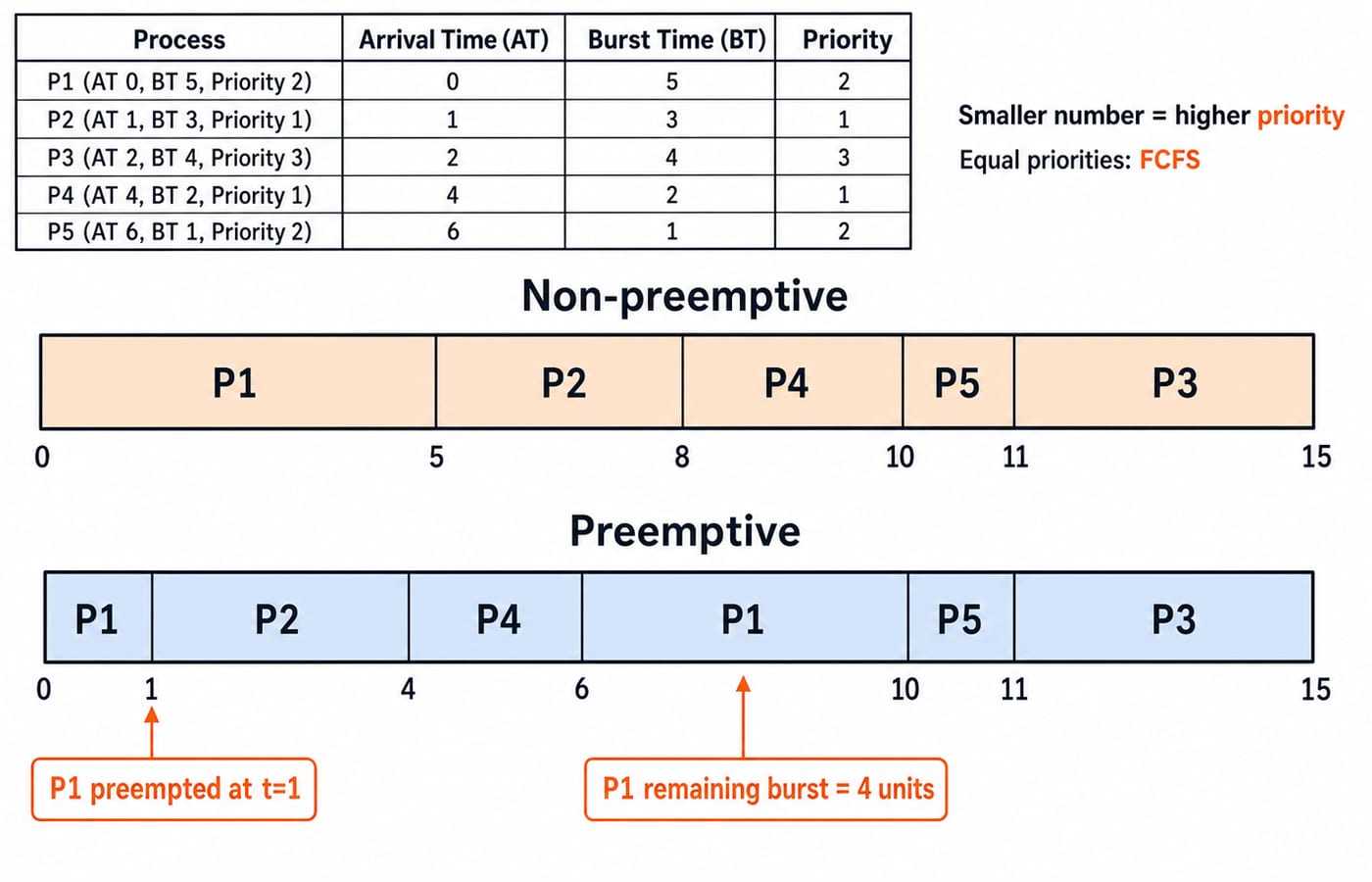
At t = 0, only P1 is ready, so it must run from 0 to 5. P2 arrives at t = 1 with higher priority, but this variant cannot interrupt P1. At t = 5, P2 and P4 are both priority 1, so earlier arrival P2 runs 5-8. P4 follows at 8-10, then P5 at 10-11, and P3 at 11-15.
Gantt chart: 0 | P1 | 5 | P2 | 8 | P4 | 10 | P5 | 11 | P3 | 15
Process | First start | CT | TAT = CT - AT | WT = TAT - BT | RT = first start - AT |
|---|---|---|---|---|---|
P1 | 0 | 5 | 5 | 0 | 0 |
P2 | 5 | 8 | 7 | 4 | 4 |
P3 | 11 | 15 | 13 | 9 | 9 |
P4 | 8 | 10 | 6 | 4 | 4 |
P5 | 10 | 11 | 5 | 4 | 4 |
Average turnaround time is (5 + 7 + 13 + 6 + 5) / 5 = 36 / 5 = 7.2 time units. Average waiting time is (0 + 4 + 9 + 4 + 4) / 5 = 21 / 5 = 4.2 time units. Response time equals waiting time in this trace because each process receives one uninterrupted CPU interval. That equality is not universal.
Preemptive priority scheduling: trace arrivals and remaining burst
Only the preemption rule changes: a smaller number means higher priority, and FCFS breaks ties.
P1 starts at t = 0. P2 arrives at t = 1 with priority 1, so it preempts P1. P1 has 5 - 1 = 4 units left. P2 runs from 1 to 4; P3 arrives at t = 2 with priority 3 and cannot preempt it. At t = 4, P2 completes as P4 arrives, so P4 runs 4-6.
At t = 6, P5 arrives with priority 2. P1 has the same priority but arrived earlier, so FCFS selects it. P1 resumes for its four remaining units from 6 to 10. P5 then runs 10-11, followed by P3 from 11 to 15.
Gantt chart: 0 | P1 | 1 | P2 | 4 | P4 | 6 | P1 | 10 | P5 | 11 | P3 | 15
Process | First start | CT | TAT | WT | RT |
|---|---|---|---|---|---|
P1 | 0 | 10 | 10 | 5 | 0 |
P2 | 1 | 4 | 3 | 0 | 0 |
P3 | 11 | 15 | 13 | 9 | 9 |
P4 | 4 | 6 | 2 | 0 | 0 |
P5 | 10 | 11 | 5 | 4 | 4 |
Average turnaround time is (10 + 3 + 13 + 2 + 5) / 5 = 33 / 5 = 6.6. Average waiting time is (5 + 0 + 9 + 0 + 4) / 5 = 18 / 5 = 3.6. Average response time is (0 + 0 + 9 + 0 + 4) / 5 = 13 / 5 = 2.6. For broader CS learning, Zero to Hero: Complete CS Course is an optional route.
Starvation and ageing: why priority needs a fairness policy
Starvation is indefinite postponement of a ready low-priority process as higher-priority work arrives. Unlike deadlock, it remains eligible but repeatedly loses selection; no circular wait is required. Ageing (also written aging) improves its priority over time.
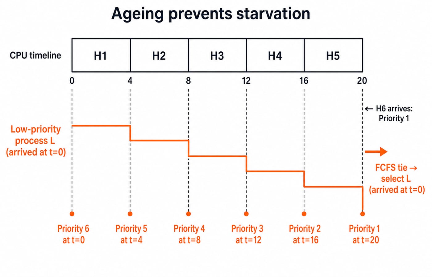
L arrives at t = 0 with priority 6 and needs 2 CPU units. H1 to H5 each have priority 1, need 4 units, and arrive at t = 0, 4, 8, 12, 16. Without ageing, a continuing stream can postpone L indefinitely.
Improve L's numeric priority by 1 after every 4 complete waiting units: 6 at t=0, 5 at t=4, 4 at t=8, 3 at t=12, 2 at t=16, and 1 at t=20. If H6 arrives at t = 20 with priority 1, FCFS selects L because it has waited since t = 0. Ageing bounds neglect under this arrival pattern, but its interval and adjustment step are policy choices, not universal constants.
Priority scheduling compared with FCFS, SJF and Round Robin
Policy | Selection key | Can preempt? | Main strength | Main risk |
|---|---|---|---|---|
FCFS | Earliest arrival | No | Simple arrival order | Convoy effect |
SJF or SRTF | Shortest burst or remaining time | SRTF can | Favours short work | Needs burst knowledge or estimation |
Round Robin | Rotating time quantum | Yes | Regular CPU turns | Quantum and context-switch trade-offs |
Priority | Importance or urgency | Either | Expresses relative importance | Starvation |
Priority and preemption are separate axes. A priority policy can be preemptive or non-preemptive, and a system can use priority classes with Round Robin inside each equal-priority class. For this workload, preemption changes average waiting from 4.2 to 3.6 and average turnaround from 7.2 to 6.6, while P1's waiting rises from 0 to 5. This single result does not make preemptive priority scheduling universally best.
Priority scheduling traps: run a six-check audit
Before calculating:
Copy priority direction.
Consider only arrived processes at each decision.
Mark whether the policy is preemptive.
Apply the stated tie-breaker.
Reduce remaining burst after an interruption.
Compute metrics from the final chart.
In the non-preemptive trace, selecting P2 at t = 1 is wrong because P1 owns the CPU until t = 5. In the preemptive trace, choosing P5 at t = 6 is wrong because P1 has the same priority and arrived first.
For either trace, sum of CPU intervals = sum of burst times = 5 + 3 + 4 + 2 + 1 = 15. No idle interval appears from t = 0 to 15 because one process is always ready. If the ready queue becomes empty, show its idle segment on the Gantt chart.
How exam questions test priority scheduling
Common forms ask for a Gantt chart, a comparison of preemptive and non-preemptive output, CT, TAT, WT or RT, or an ageing correction for starvation. Take the numerical priority convention and tie rule from the question.
Use this quick method: first annotate the convention and draw the arrival-event times. Maintain a ready list as (process, priority, remaining burst). Choose only at a legal scheduling point, and record CT immediately when a process ends. Then derive TAT and WT in a separate table. This separates scheduling decisions from arithmetic and makes mistakes easier to find.
Next, test the method on Process Scheduling MCQs: 12 Solved (GATE).
Priority scheduling in the short version
Define the priority direction, distinguish preemptive from non-preemptive selection, resolve every tie, carry the remaining burst after preemption, and check starvation before calling a policy fair. This workload gives average waiting times of 4.2 non-preemptively and 3.6 preemptively, not a universal ranking. GATE Guidance by Sanchit Sir is an optional structured route for the wider GATE CS syllabus. Otherwise, redraw both timelines from a blank table and attempt the linked scheduling MCQs.
Go deeper with the full courseOperating System
Keep learning
Process Management in Operating Systems: States, PCB and Scheduling Worked Examples
Connect the process lifecycle, PCB, queues and dispatcher, then calculate FCFS and Round Robin metrics through one complete scheduling example.
Updated 29 Aug 20266 min readOperating Systems

Operating Systems for GATE: How to Study Deadlocks, Scheduling and Memory
Operating Systems is one of the densest, most-tested GATE CS subjects. Here is how to study its three biggest areas (scheduling, deadlocks and memory) so the marks actually come.
Updated 26 Jul 202610 min read199 viewsOperating Systems
ISRO CS Operating Systems PYQ Patterns: Scheduling, Memory and Deadlock Worked Step by Step
Learn four scratch-work methods for ISRO-style Operating Systems problems. Follow complete Round Robin, paging, LRU, semaphore and deadlock safety traces.
Updated 17 Aug 20266 min read156 viewsISRO Recruitment

Operating System Scenarios: Solve Scheduling, Concurrency, and Page Replacement
Learn one state-trace method for three common OS problem families, then apply it to complete Round Robin, concurrency, FIFO, and LRU examples.
Updated 30 Oct 20265 min readOperating Systems