

Randomized Algorithms Explained: Las Vegas, Monte Carlo and a Worked Quicksort Trace
Learn what random choices change in an algorithm, then trace randomized quicksort and calculate its expected comparisons and repeated-trial error.
KnowledgeGate Team
Exam prep & CS education
Updated 4 Nov 20266 min read

Random choices do not all buy the same guarantee. Randomized quicksort always returns a sorted result while pivot choices change its comparison count. A Monte Carlo test can instead trade a quantified chance of error for bounded work, and independent repetition reduces that error multiplicatively.
1. What makes an algorithm randomized
A randomized algorithm uses random bits or choices alongside the input. For fixed input I, seeds can change execution paths, running times or outputs. Average-case analysis instead places a probability distribution over inputs.
For [7,2,5,1,6,3,4], deterministic first-element quicksort must take pivot 7. Randomized quicksort can choose any of the seven positions, each with probability 1/7. The rule must say "uniformly at random" because "choose a pivot" defines no distribution.
Randomization can reduce dependence on adversarial input order and simplify analysis, but an expected bound remains no per-run guarantee. For wider syllabus revision, use GATE CS Exam Preparation Courses and Test Series.
2. Las Vegas and Monte Carlo are different promises
The two families place uncertainty in different parts of the promise.
Family | Answer guarantee | Resource guarantee | Example |
|---|---|---|---|
Las Vegas | Returned answer is always correct | Running time or work is random | Randomized quicksort on distinct keys |
Monte Carlo | Answer may be wrong with a quantified probability | Work is bounded for the stated trial count | Randomized compositeness or fingerprint test |
Ask: Can the output be wrong? If no but runtime varies, think Las Vegas; if yes with bounded error, think Monte Carlo. One-sided error makes one answer conclusive; with two-sided error, either answer may be wrong within its bound.
Correctly implemented randomized quicksort always sorts. Only comparisons depend on the pivots. A slow sequence changes work, not correctness, making it Las Vegas rather than Monte Carlo.
3. The probability toolkit: random variables, expectation and independence
Let C count key comparisons on one fixed input. E[C] is their probability-weighted average across pivot sequences, not one observed run or an exact per-run count.
For seven distinct ranks, a first pivot from the middle three ranks {3,4,5} has probability 3/7; an extreme first pivot from {1,7} has probability 2/7. If two independent choices fail with probabilities p and q, both fail with probability pq. That multiplication requires independence.
An indicator X is 1 when an event occurs and 0 otherwise, so E[X] = Pr(X=1). Linearity gives E[X_1 + ... + X_k] = E[X_1] + ... + E[X_k] even for dependent indicators, letting us add pairwise comparison probabilities.
4. Randomized quicksort: the algorithm before the arithmetic
For distinct keys, sizes 0 or 1 return immediately. Otherwise, choose one position uniformly at random as p. Compare every other key with p, put smaller keys in L and larger keys in R, recursively sort both, then return quicksort(L) + [p] + quicksort(R). A size-m partition makes exactly m-1 key comparisons.
For seven distinct keys, encounter order inside L and R is preserved, recursive calls run left before right, and no pivot is drawn in base cases. For duplicates, use an explicit equality or three-way-partition rule.
Randomized pivot selection changes quicksort's comparison path; Sorting Algorithms: Complexity and Comparison compares time, space and stability across sorting methods.
5. Worked example: sort seven keys with three recorded random draws
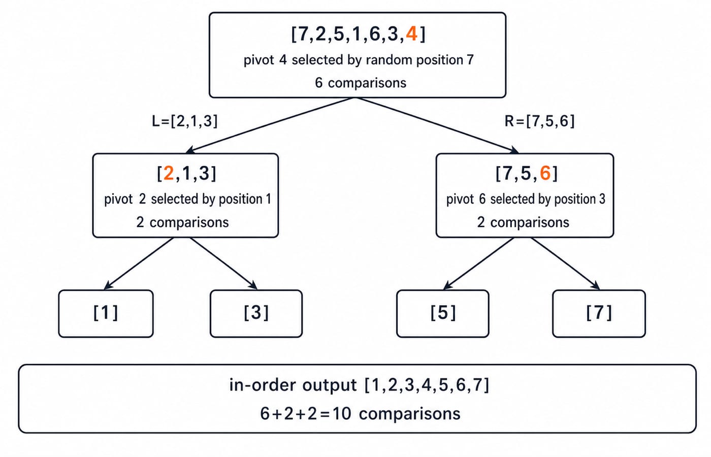
Start with [7,2,5,1,6,3,4] and use the successive 1-indexed random-position draws [7,1,3].
Call | Current keys | Random position | Pivot | L | R | New comparisons | Running total |
|---|---|---|---|---|---|---|---|
Root |
| 7 | 4 |
|
| 6 | 6 |
Left |
| 1 | 2 |
|
| 2 | 8 |
Right |
| 3 | 6 |
|
| 2 | 10 |
The root draw selects 4. Comparing it with the other six keys produces L=[2,1,3] and R=[7,5,6]. Next, the left call selects 2 and makes two comparisons. Its children are [1] and [3]. The right call then selects 6, makes two comparisons, and produces [5] and [7]. Every remaining call is a one-element base case. Each row follows the rule that a size-m partition uses m-1 comparisons.
The nested result is ([1]+[2]+[3]) + [4] + ([5]+[6]+[7]), which equals [1,2,3,4,5,6,7]. The total is 6+2+2=10 comparisons. Under independent uniform draws, the conditional probability of exactly this recorded pivot path is (1/7)(1/3)(1/3)=1/63. That is the probability of this path, not the probability that quicksort is correct.
6. Why the expected comparison count is Theta(n log n)
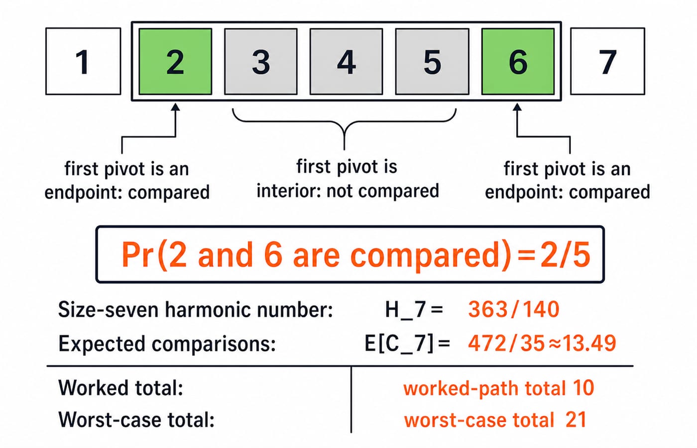
Write the distinct sorted ranks as z_1 < ... < z_n. Let X_ij=1 if z_i and z_j are ever compared. This pair is compared exactly when the first pivot chosen from the contiguous block {z_i,...,z_j} is one of its two endpoints. The block contains j-i+1 possible first pivots, so Pr(X_ij=1)=2/(j-i+1).
For example, ranks 2 and 6 define a five-rank block. They are compared with probability 2/5, because the block's first pivot must be 2 or 6.
Linearity of expectation now gives
E[C_n] = sum_{1 <= i < j <= n} E[X_ij] = sum_{1 <= i < j <= n} 2/(j-i+1) = 2(n+1)H_n - 4n,
where H_n=1+1/2+...+1/n. For n=7, H_7=363/140. Therefore
E[C_7] = 16(363/140) - 28 = 472/35, about 13.49 comparisons.
This expectation is over the internal pivot choices for the fixed input. Our recorded run used 10 comparisons. A worst-case chain of extreme pivots uses 6+5+4+3+2+1=21. Thus the expected comparison count is Theta(n log n), while the worst case remains Theta(n^2). One 10-comparison run does not prove the expected bound, and it does not contradict an expectation of about 13.49.
7. Monte Carlo error amplification and the traps it exposes
Suppose a one-sided Monte Carlo test has this promise: every reported witness is valid, but on an input that has a witness, one trial can miss it with probability at most 1/4. Run five trials with fresh independent randomness and stop when a witness appears. All five miss with probability at most (1/4)^5=1/1024, about 0.0977%. The work grows by at most a factor of 5.
Seeing a witness is conclusive under this promise; five misses do not make the opposite answer certain. Two-sided error needs a different majority-voting calculation, so do not reuse the all-fail formula without checking the rule.
Remember:
Randomized does not mean unanalysed.
Expected time is not worst-case time.
Las Vegas may be slow but does not trade correctness for speed.
Monte Carlo has bounded error, not an unspecified guess.
Multiplying failures requires fresh independent trials.
Fixing one seed reproduces a bug but is not repeated independent testing.
8. How questions test the topic, the short version and the next step
Questions may ask you to classify a promise as Las Vegas or Monte Carlo, find a pivot probability, trace a random-index sequence, count comparisons, separate expected from worst-case complexity, apply 2/(j-i+1), or amplify an independent one-sided error bound.
Use the GATE Test Series: Mocks and Topic-wise Tests for timed classification, trace and probability practice.
On a fresh problem, classify what randomness changes: runtime, the returned answer, or both. For a quicksort trace, record the pivot, subarrays and m-1 comparisons at each non-base call. For amplification, define the single-trial failure event before multiplying independent probabilities.
Recreate the 6+2+2=10 trace without looking and explain why E[C_7]=472/35 does not contradict it. Continue through GATE Guidance by Sanchit Sir for a structured route, and use Dynamic Programming Explained: 0/1 Knapsack as the next algorithm-design topic.
Keep learning
Matrix Chain Order: DP Recurrence, Table and a 4-Matrix Worked Example
See why order changes scalar cost even when the final matrix does not. Build both DP tables for p = [5, 10, 3, 12, 5] and recover the 405-cost solution.
Updated 10 Nov 20266 min readDSA & Algorithms

Longest Common Subsequence (LCS): Build the DP Table Step by Step
Build an LCS table from its prefix state, trace every important cell, and backtrack one valid answer. The worked example ends with GTAB.
Updated 9 Nov 20265 min readDSA & Algorithms

Fractional Knapsack Explained: Greedy Logic, Worked Example and Exam Traps
Learn why ratio order is optimal for divisible items, trace every step of a capacity-50 solution, and avoid common greedy and arithmetic mistakes.
Updated 8 Nov 20266 min readDSA & Algorithms

Growth Rate Comparisons: How to Order Functions Step by Step
Learn how to normalise and order logarithmic, polynomial, exponential, and factorial functions without letting a small-value table mislead you.
Updated 6 Nov 20265 min readDSA & Algorithms