

Fractional Knapsack Explained: Greedy Logic, Worked Example and Exam Traps
Learn why ratio order is optimal for divisible items, trace every step of a capacity-50 solution, and avoid common greedy and arithmetic mistakes.
KnowledgeGate Team
Exam prep & CS education
Updated 8 Nov 20266 min read

Fractional knapsack differs from 0/1 knapsack because divisible items change the optimisation method. The value-to-weight greedy rule assigns capacity to the highest value density. For capacity 50, items A(10, 60), B(20, 100), and C(30, 120) give fractional value 240 but 0/1 value 220. The GATE CS Exam Preparation Courses & Test Series path connects related algorithms, while GATE Guidance by Sanchit Sir provides a structured sequence.
Define the fractional knapsack problem precisely
There are n items. Item i has positive weight w_i and positive value v_i, while the knapsack has capacity W. We may choose a fraction x_i where 0 <= x_i <= 1.
The constraint is sum(x_i * w_i) <= W, and the objective is to maximise sum(x_i * v_i). Dividing an item scales its weight and value proportionally. For example, taking half of an item uses half its weight and earns half its value.
Fractional knapsack permits a choice such as x_i = 2/3; 0/1 knapsack restricts each x_i to 0 or 1.
Define an item's density, or value-to-weight ratio, as r_i = v_i / w_i. An item with weight 4 and value 28 has ratio 28/4 = 7, so every unit of capacity assigned to it contributes 7 units of value.
Explain why the highest ratio must come first
Capacity is the scarce resource. Each unit should therefore be assigned to the available item that gives the highest value per unit of weight. Sorting by total value ignores capacity consumed, while sorting by weight ignores the return from that weight.
An exchange argument makes the choice precise. Suppose a solution uses positive weight from an item with ratio r_low while some higher-ratio item with r_high > r_low remains available. Let delta be the smaller of the low-ratio weight used and the high-ratio weight still available. Moving delta weight units to the higher-ratio item changes the value by delta * (r_high - r_low), which is positive. A solution containing such an inversion cannot be optimal.
Therefore, sort items by descending ratio, take complete items while they fit, then take exactly enough of the first non-fitting item to fill the remaining capacity. Equal-ratio items may appear in either order because they give the same value per capacity unit.
The capacity-50 A-B-C benchmark also appears in Greedy Algorithms for GATE CS: Concepts, Worked Examples, and Where Greedy Fails, where it is one example inside a six-problem survey. In fractional knapsack, the same benchmark supports the full exchange proof, step-by-step fraction trace, feasibility check, pseudocode state, and exact contrast with 0/1 selection.
Work the capacity-50 example from ratios to final value
Let W = 50 and use these items:
Item | Weight | Value | Ratio |
|---|---|---|---|
A | 10 | 60 |
|
B | 20 | 100 |
|
C | 30 | 120 |
|
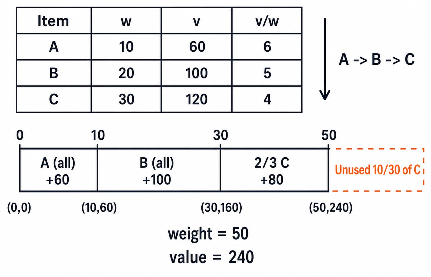
The descending ratio order is A, B, C.
Take all of
A. Used weight is10, remaining capacity is50 - 10 = 40, and total value is60.Take all of
B. Used weight is10 + 20 = 30, remaining capacity is40 - 20 = 20, and total value is60 + 100 = 160.Only
20ofC's30weight units fit. Take fraction20/30 = 2/3, adding(2/3) * 120 = 80. Used weight becomes50, remaining capacity becomes0, and final value is60 + 100 + 80 = 240.
Feasibility follows from the selected fractions x_A = 1, x_B = 1, and x_C = 2/3: 1*10 + 1*20 + (2/3)*30 = 10 + 20 + 20 = 50. Their value is 1*60 + 1*100 + (2/3)*120 = 60 + 100 + 80 = 240. Optimality follows from the ratio-order exchange argument, not merely from trying one convenient order.
Turn the rule into an algorithm and analyse its cost
for each item:
    item.ratio = item.value / item.weight
sort items by descending ratio
remaining = W
total = 0
fractions = all zeros
for each item in sorted order:
    if item.weight <= remaining:
        fractions[item] = 1
        total = total + item.value
        remaining = remaining - item.weight
    else:
        fraction = remaining / item.weight
        fractions[item] = fraction
        total = total + fraction * item.value
        remaining = 0
        stop
return total, fractions
On the example, the state (remaining, total) becomes (40, 60) after A, (20, 160) after B, and (0, 240) after 2/3 of C. At most one item is fractional because the first partial item consumes all remaining capacity.
Computing ratios costs O(n), sorting costs O(n log n), and selection costs O(n), giving O(n log n) total time. If the items are already ratio-sorted, selection is O(n). Auxiliary space depends on the sorting implementation and whether new item records are created.
Separate fractional knapsack from 0/1 knapsack
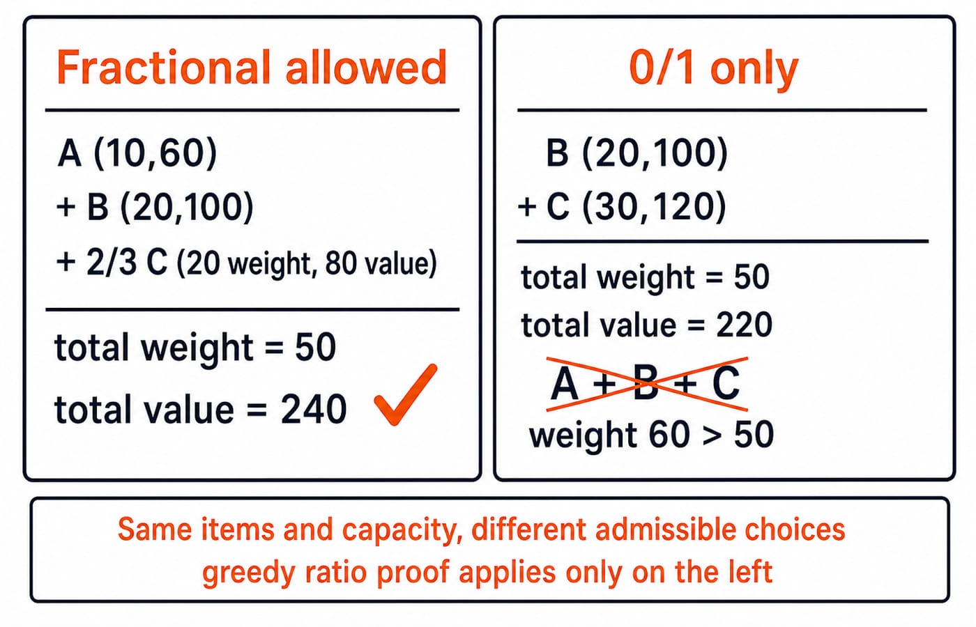
For the same capacity-50 input, fractional knapsack selects A + B + 2/3 of C for value 240. The non-empty complete-item choices in 0/1 knapsack are:
Choice | Weight | Value | Result |
|---|---|---|---|
A | 10 | 60 | Feasible |
B | 20 | 100 | Feasible |
C | 30 | 120 | Feasible |
A + B | 30 | 160 | Feasible |
A + C | 40 | 180 | Feasible |
B + C | 50 | 220 | Best feasible |
A + B + C | 60 | 280 | Infeasible |
Thus the best 0/1 value is 220 from B + C, not 240. The exchange proof works only when an arbitrary amount of weight can move between divisible items. With indivisible items, taking the locally highest ratio can block a better complete-item combination.
For the corresponding whole-item method, study the Dynamic Programming Explained with a Worked 0/1 Knapsack. Fractional knapsack itself does not need a dynamic-programming table.
Diagnose the traps that produce a wrong greedy answer
Sorting by raw value
Value order is C(120), B(100), A(60). Taking C and then B fills weight 30 + 20 = 50 for value 120 + 100 = 220, losing 240 - 220 = 20 against ratio order.
Sorting by smallest weight
For capacity 10, let P(w=2,v=4,r=2), Q(w=3,v=5,r=5/3), and R(w=8,v=80,r=10). Weight-first takes P and Q, then 5/8 of R, earning 4 + 5 + (5/8)*80 = 4 + 5 + 50 = 59. Ratio-first takes R and then P, earning 80 + 4 = 84.
Arithmetic and model slips
Calculate remaining/item_weight, not the reverse. Multiply the chosen fraction by both weight and value, stop when capacity reaches zero, and retain exact fractions such as 2/3 until the final display. Before calculating, check whether the problem allows fractions or requires 0/1 decisions.
Recognise the common exam-style question forms
Exam-style questions on fractional knapsack recur in a small number of standard forms:
With the main items and
W = 40, takeA,B, and10/30 = 1/3ofC. Value is60 + 100 + (1/3)*120 = 60 + 100 + 40 = 200.With
W = 25, takeAand15/20 = 3/4ofB. Value is60 + (3/4)*100 = 60 + 75 = 135.Which change breaks the proof? Restricting every choice to whole items, because an exchange may then fail to preserve feasibility.
For
nunsorted items, the ratio and selection scans are linear, but descending comparison sorting dominates, givingO(n log n). For a pre-sorted list, scanning until capacity fills isO(n)in the worst case.
Keep the short version, then practise the decision sequence
Recall five steps: confirm divisibility, calculate value/weight, sort descending, take full items followed by one final fraction, then verify total weight and value. In the capacity-50 example, that gives A + B + 2/3 C, weight 50, value 240.
Practice 1: Capacity is
12, withX(w=4,v=20,r=5),Y(w=6,v=24,r=4), andZ(w=8,v=24,r=3). TakeX,Y, and2/8 = 1/4ofZ, for value20 + 24 + (1/4)*24 = 20 + 24 + 6 = 50.Practice 2: Two available items both have ratio
5. Swapping their order does not change value gained per capacity unit, although the recorded fractions may differ.
Use the GATE Test Series: Mocks & Topic-wise Tests as an optional route for broader practice. For a wider preparation sequence, return to the GATE Guidance course linked in the introduction.
Keep learning
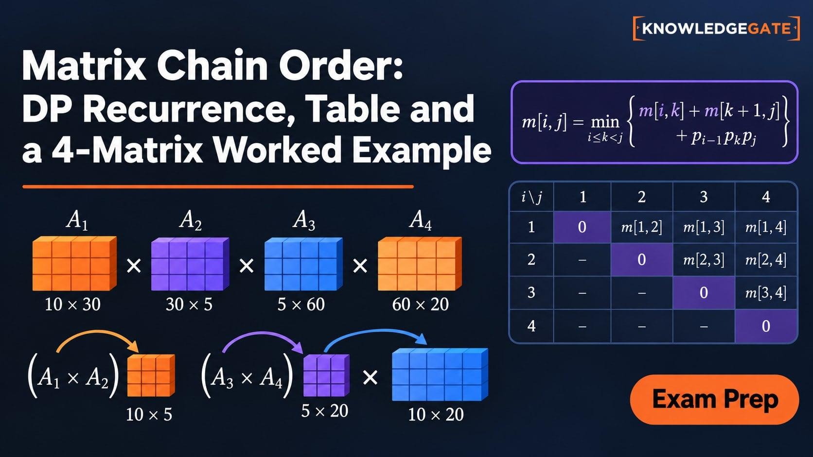
Matrix Chain Order: DP Recurrence, Table and a 4-Matrix Worked Example
See why order changes scalar cost even when the final matrix does not. Build both DP tables for p = [5, 10, 3, 12, 5] and recover the 405-cost solution.
Updated 10 Nov 20266 min readDSA & Algorithms
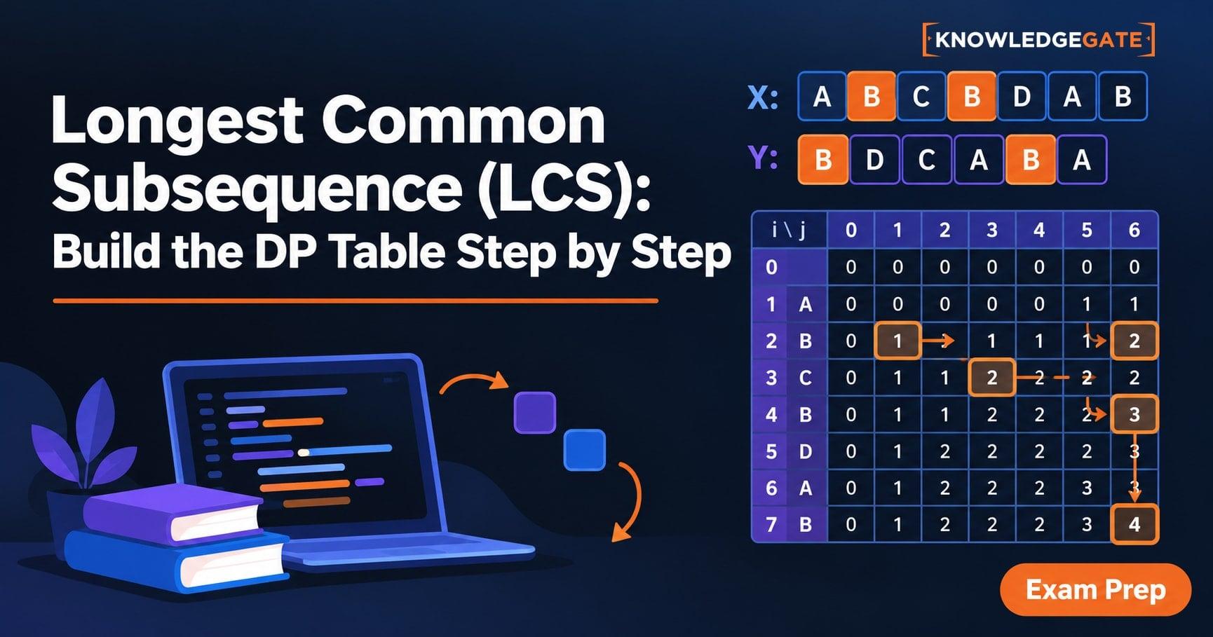
Longest Common Subsequence (LCS): Build the DP Table Step by Step
Build an LCS table from its prefix state, trace every important cell, and backtrack one valid answer. The worked example ends with GTAB.
Updated 9 Nov 20265 min readDSA & Algorithms

Growth Rate Comparisons: How to Order Functions Step by Step
Learn how to normalise and order logarithmic, polynomial, exponential, and factorial functions without letting a small-value table mislead you.
Updated 6 Nov 20265 min readDSA & Algorithms

String Matching Algorithms Explained: Naive Search, KMP and Rabin-Karp
Learn how naive search, KMP, Rabin-Karp and related methods differ. Build an LPS array, trace KMP through mismatches and verify a rolling-hash collision.
Updated 5 Nov 20266 min readDSA & Algorithms