

Algorithm Analysis Basics: Operation Counts, Growth Rates and Worked Examples
Learn to choose an input size, count operations exactly, simplify the result with asymptotic notation, and avoid common time and space analysis mistakes.
KnowledgeGate Team
Exam prep & CS education
Updated 3 Nov 20266 min read

An operation count is only as sound as the event being counted. A loop body, comparison, condition test, and index update produce different exact totals even when they reduce to the same asymptotic class. Name the input size and cost model, build an exact ledger, and simplify only after the count is complete.
Formal notation, recursion, and the Master theorem are developed in Time Complexity: Big-O, Theta, Omega and Master Theorem. Exact bookkeeping starts one level lower: choose an event, include or exclude loop machinery explicitly, and keep the exact answer separate from its growth class.
Define the input size, algorithm, and counted event
A problem states a required result. An algorithm is a finite, unambiguous sequence that maps valid input to that result; C, Java, or Python code is one implementation. Analysis begins with the algorithm and input size, not one stopwatch reading.
For A = [7, 3, 11, 5, 9], a maximum scan sets largest = A[0] and compares each remaining element with the current maximum. The comparisons are 3 > 7, 11 > 7, 5 > 11, and 9 > 11. The output is 11 after exactly n - 1 = 4 comparisons. Counting assignments as well would produce a different exact total, so the event must be named.
Use n elements for an array, V vertices and E edges for a graph, and bit length for an integer. A RAM-style model treats a chosen elementary operation as constant cost. Machine, language, and compiler still affect seconds, but they do not change the count as a function of input size. The GATE CS preparation category connects this analysis to the wider subject path.
Build an exact ledger for a geometric nested loop
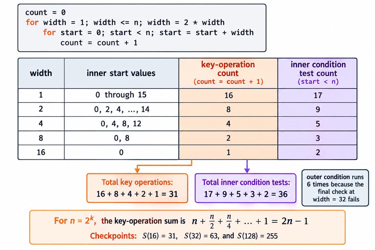
Declare count = count + 1 as the key operation. The inner step size depends on the outer width:
count = 0
for width = 1; width <= n; width = 2 * width
    for start = 0; start < n; start = start + width
        count = count + 1
At n = 16, the widths are 1, 2, 4, 8, 16. The inner loop visits fewer positions each time:
width | start values | Key-operation count | Inner condition tests |
|---|---|---|---|
1 | 0 through 15 | 16 | 17 |
2 | 0, 2, 4, ..., 14 | 8 | 9 |
4 | 0, 4, 8, 12 | 4 | 5 |
8 | 0, 8 | 2 | 3 |
16 | 0 | 1 | 2 |
The declared key operation runs 16 + 8 + 4 + 2 + 1 = 31 times. Inner condition tests run 17 + 9 + 5 + 3 + 2 = 36 times, and the outer condition runs 6 times because the final check at width = 32 fails. None of those totals can replace another unless the question changes the cost model.
For n = 2^k, the key-operation sum is n + n/2 + n/4 + ... + 1 = 2n - 1. Thus S(16) = 31, S(32) = 63, and S(128) = 255. For non-powers of two, ceilings appear in the rows, but the total remains bounded by a constant multiple of n.
Algorithm Analysis: Asymptotic Notation, Recurrences and Worked Examples for GATE CS uses a triangular loop, a merge-sort recurrence tree, and a dynamic-array amortized trace. The geometric ledger tests a different mistake: nested syntax can still produce linear total work when the inner range shrinks as the outer width doubles.
Convert the exact ledger to O, Omega, and Theta
O(g(n)) is an asymptotic upper bound, Omega(g(n)) is a lower bound, and Theta(g(n)) gives matching upper and lower bounds. For the geometric ledger and every n >= 1 that is a power of two,
n <= 2n - 1 <= 2n.
Constant multiples of n bound the exact count on both sides, so S(n) = Theta(n). It is also O(n^2), but that upper bound is loose. Constants and lower-order terms may be dropped for an asymptotic class, never for an exact-count answer such as S(16) = 31.
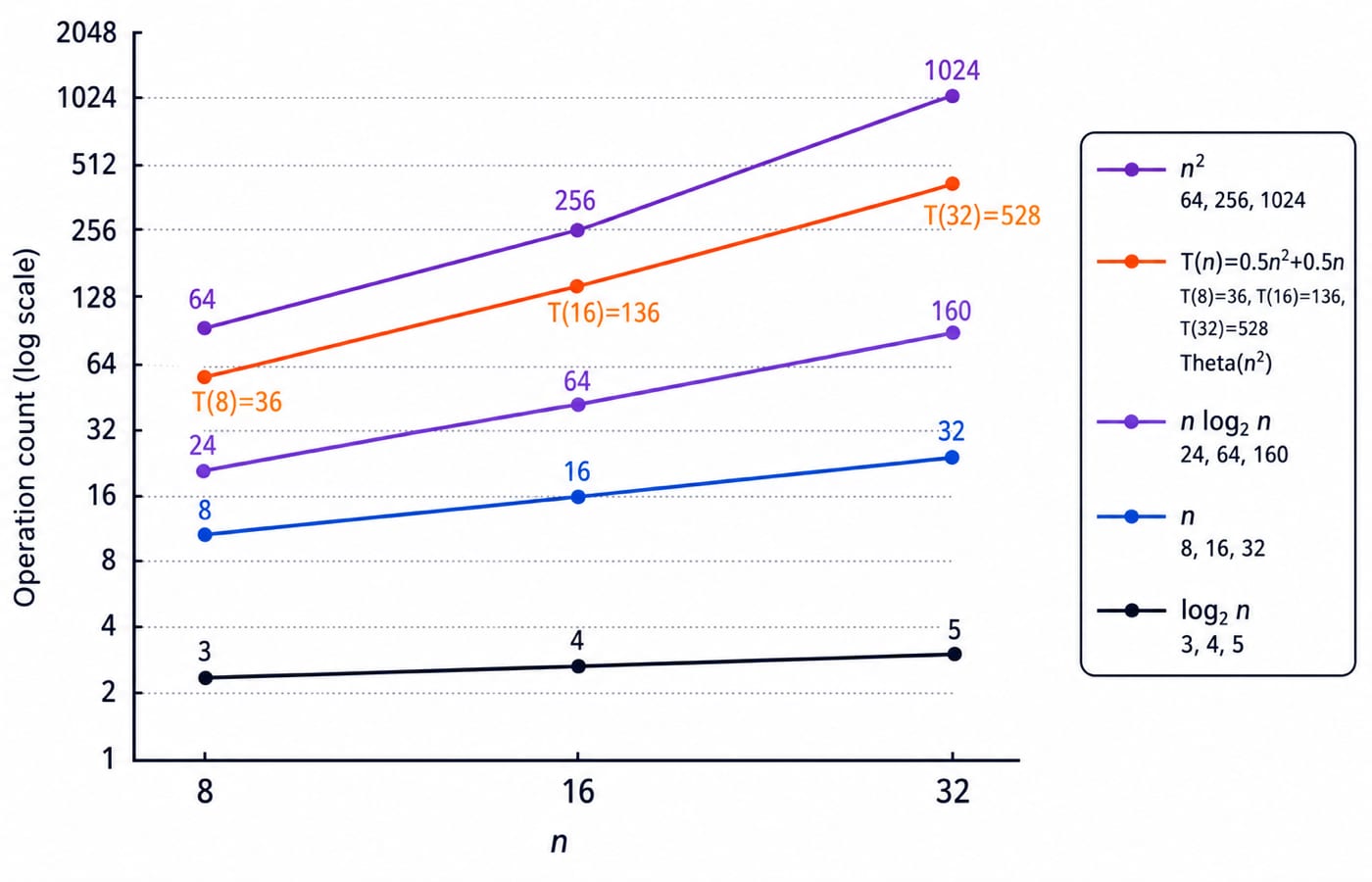
Contrast that result with a triangular loop whose row lengths are 1, 2, ..., n. Its exact count is T(n) = n(n + 1)/2, giving T(8) = 36, T(16) = 136, and T(32) = 528. The two pieces of code are both nested, yet one is linear and the other quadratic because their dependent ranges sum differently.
Keep best, worst, and average cases separate
Consider an early-exit scan for zero. On [0, 9, 2, 7, 5], it stops after 1 comparison. On [4, 9, 2, 7, 0], it needs 5, and an array with no zero also needs 5. The best case is Theta(1) and the worst case is Theta(n).
If a successful target is equally likely to appear in any of the n positions, the expected comparison count is (1 + 2 + ... + n)/n = (n + 1)/2. At n = 5, that is 3. Without the distribution assumption, an average-case number is unsupported. An unsuccessful scan still takes exactly n comparisons.
Best, average, and worst choose an input or distribution. O, Omega, and Theta bound the resulting function. Time Complexity Analysis of Algorithms: Big-O, Recurrences, and Worked Examples extends the calculation to four loop patterns, merge sort, quicksort cases, and counts at 10 and 1000 elements. The early-exit scan isolates the distribution assumption that makes an average meaningful.
Separate input, output, and auxiliary space
The geometric ledger stores width, start, and count beyond its input, so its auxiliary space is Theta(1). Copying an n-element array before scanning needs Theta(n) auxiliary space. Returning a required n-element result uses Theta(n) output space, which should be reported separately when the question excludes output from auxiliary memory.
Recursion depth also occupies auxiliary space. Let sum(A, m) call sum(A, m - 1) until m = 0. Starting at m = 5 creates active calls for 5, 4, 3, 2, 1, 0, so the maximum is 6 frames. In general the depth is n + 1, which is Theta(n) stack space even when each frame stores only constant local state.
Avoid loop-counting traps that change the answer
Do not multiply every visual nesting. The geometric loop at
n = 16performs 31 key operations, not16 * 5 = 80, because the inner count shrinks.Add sequential blocks. Counts of
3nand2ntotal5n = Theta(n).Multiply independent nested ranges. An
n-iteration outer loop containing a fulllog n-iteration inner loop costsTheta(n log n).Count the values of a multiplicative loop. Starting from 32 and halving gives
32, 16, 8, 4, 2, 1, or 6 iterations.Distinguish input value from input size. The value
N = 1024needs 11 binary bits, so a loop from 1 through 1024 is exponential in the bit length.
Solve exact checkpoints before naming a growth class
For the geometric nested loop at
n = 8, count8 + 4 + 2 + 1 = 15key operations, so the class isTheta(n).For triangular row lengths through
n = 12, calculate12 * 13 / 2 = 78before reportingTheta(n^2).For
j = 1; j <= 81; j *= 3, list1, 3, 9, 27, 81. There are 5 body executions and logarithmic growth.From slower to faster eventual growth, order
log n, sqrt(n), n, n log n, n^2, 2^n.
Operation counting: the compact audit sequence
Define the input size.
Choose the counted event.
List changing values or row lengths.
Include loop tests and updates only when the cost model asks for them.
State the best, worst, or assumed average case.
Simplify to a tight asymptotic class and report auxiliary space separately.
The central ledger has three useful checkpoints: S(16) = 31 key operations, 36 inner condition tests, and S(n) = 2n - 1 = Theta(n) for powers of two. Those values catch the common but incorrect Theta(n log n) answer based only on the two loop headers.
For timed mixed practice, use the GATE Test Series: Mocks and Topic-wise Tests after reproducing the geometric and triangular counts without looking at the formulas.
Keep learning
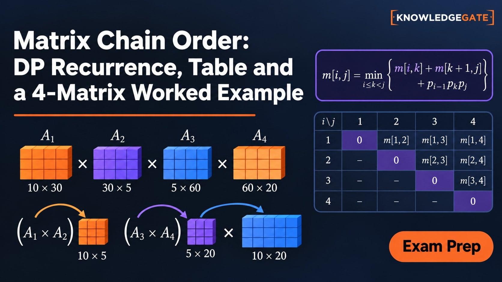
Matrix Chain Order: DP Recurrence, Table and a 4-Matrix Worked Example
See why order changes scalar cost even when the final matrix does not. Build both DP tables for p = [5, 10, 3, 12, 5] and recover the 405-cost solution.
Updated 10 Nov 20266 min readDSA & Algorithms
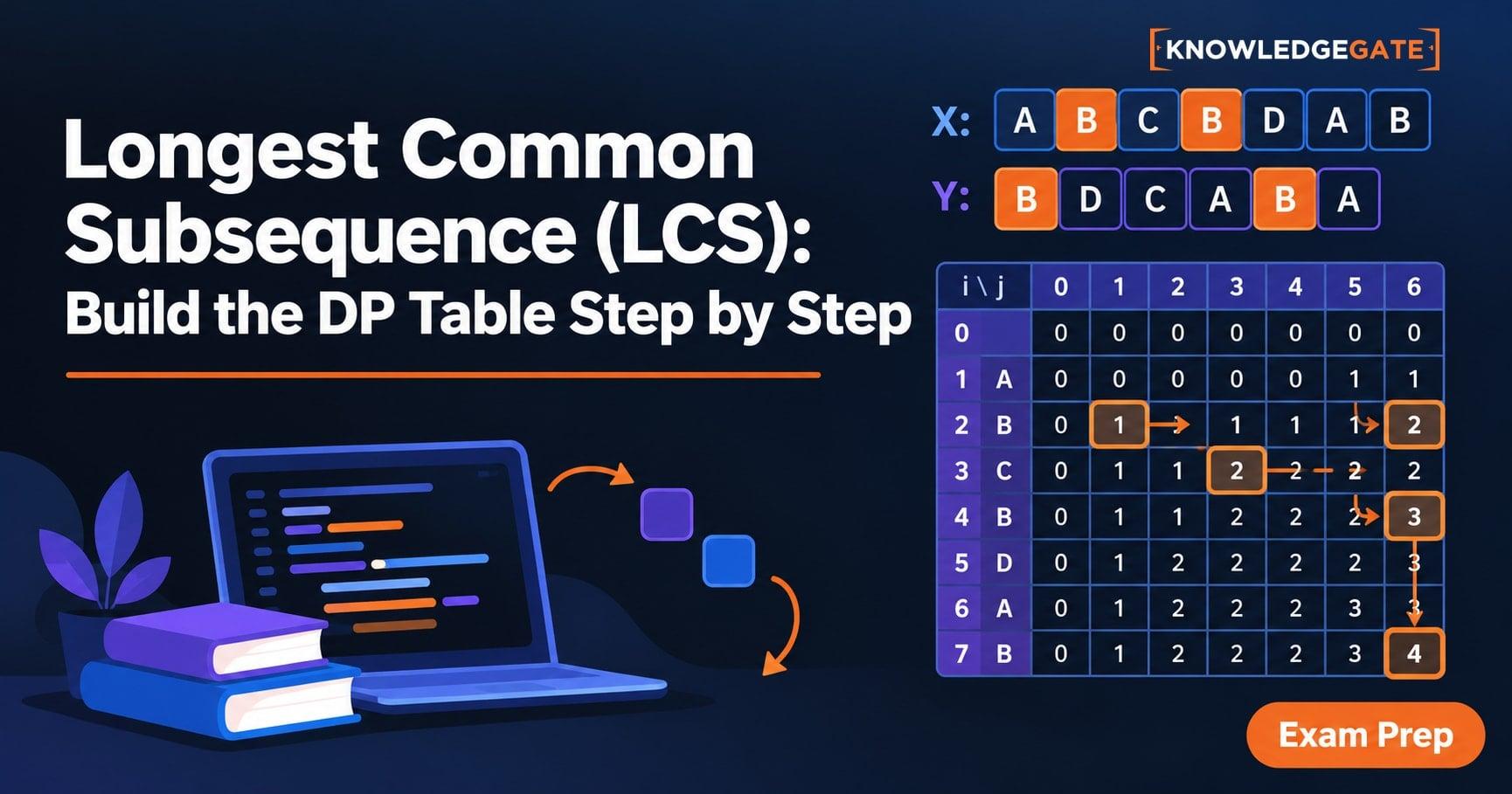
Longest Common Subsequence (LCS): Build the DP Table Step by Step
Build an LCS table from its prefix state, trace every important cell, and backtrack one valid answer. The worked example ends with GTAB.
Updated 9 Nov 20265 min readDSA & Algorithms
Fractional Knapsack Explained: Greedy Logic, Worked Example and Exam Traps
Learn why ratio order is optimal for divisible items, trace every step of a capacity-50 solution, and avoid common greedy and arithmetic mistakes.
Updated 8 Nov 20266 min readDSA & Algorithms
Growth Rate Comparisons: How to Order Functions Step by Step
Learn how to normalise and order logarithmic, polynomial, exponential, and factorial functions without letting a small-value table mislead you.
Updated 6 Nov 20265 min readDSA & Algorithms