

Data Link Layer Flow Control: Stop-and-Wait, Sliding Windows and Worked Numericals
Build a reliable method for DLL flow-control problems by tracing one link from frame timing to windows, receiver credit, sequence-space limits and ACK policy.
KnowledgeGate Team
Exam prep & CS education
Updated 12 Nov 20266 min read

Flow-control questions often mix frame size, link rate, propagation, acknowledgements, receiver capacity and sequence numbers. A remembered formula can therefore solve the wrong model. Stop-and-Wait and sliding windows determine the link's timing and utilisation, while sequence space and piggybacking affect its correctness and overhead. Each numerical value is an explicit assumption in the textbook model. Data Link Layer flow control remains distinct from error recovery and transport-layer congestion control.
Data Link Layer flow control limits data in flight
Flow control matches outstanding data, sent but not yet acknowledged, to what the receiver and link can support. Stop-and-Wait permits one outstanding frame. A sliding window permits several and advances as ACKs arrive.
Idea | Role in the model |
|---|---|
Sender window | Frames permitted outstanding |
Receiver capacity | Available input buffer |
ACK | Confirms reception and advances the window |
Sequence number | Distinguishes frames across wraparound |
Transmission delay | Time to place a frame on the link |
Propagation delay | Travel time between endpoints |
Piggybacking | ACK carried with reverse data |
The usable allowance is the smaller active limit. Flow control prevents receiver overrun, error control handles damage or loss, and congestion control responds to network overload. Shared ACKs and windows do not make them the same mechanism. The CS Fundamentals map places this distinction among related concepts.
One timing model exposes the Stop-and-Wait cost
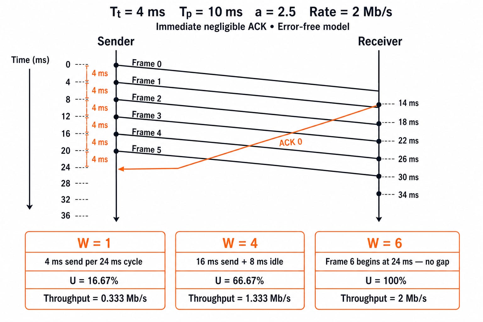
Use a full-duplex point-to-point link with a 1,000-byte = 8,000-bit frame, rate R = 2 Mb/s, and one-way propagation T_p = 10 ms. ACK transmission and processing are negligible. There are no errors, and the receiver has enough buffer unless stated otherwise.
Transmission delay is:
T_t = L/R = 8,000/(2 x 10^6) = 0.004 s = 4 ms
Therefore a = T_p/T_t = 10/4 = 2.5. Starting at t = 0, frame transmission ends at 4 ms. Its last bit reaches the receiver at 14 ms, and the immediate ACK returns at 24 ms. Thus:
T_cycle = T_t + 2T_p = 4 + 20 = 24 msU = T_t/T_cycle = 4/24 = 1/6 = 16.67%Useful throughput
= 8,000/0.024 = 333,333 bit/s, about0.333 Mb/s
The sender serialises for 4 ms and waits 20 ms for propagation and feedback. If ACK transmission or processing time is supplied, add it to this denominator.
Sliding windows keep the link busy
Now send six frames back to back. Frames 0 to 5 occupy sender intervals 0-4, 4-8, 8-12, 12-16, 16-20 and 20-24 ms. Their last bits arrive at 14, 18, 22, 26, 30 and 34 ms. ACK 0 returns at 24 ms, exactly when frame 5 finishes, so frame 6 can begin without a gap.
For this error-free, negligible-ACK model, the full-pipe condition is:
W >= 1 + 2a = 1 + 2(2.5) = 6
With W = 4, four frames take 16 ms, followed by an 8 ms wait for ACK 0. Utilisation is min(1, W/(1+2a)) = 4/6 = 66.67%, giving 1.333 Mb/s. With W = 6, utilisation is 100% and throughput reaches 2 Mb/s. A larger window cannot exceed the link rate. This assumes fixed full-size frames, immediate ACKs, no headers, no errors and a ready receiver.
Receiver capacity can lower the usable window
Six frames represent 6 x 8,000 = 48,000 bits outstanding. The round-trip propagation product is R x 2T_p = 2 x 10^6 x 0.020 = 40,000 bits, or five frames. One more frame can be on the transmitter while feedback travels, so this convention gives 1 + 2a = 6.
If the path can use six frames but the receiver advertises room for three, the sender uses min(6,3) = 3 frames, or 3,000 bytes. Then U = 3/6 = 50% and throughput is 1 Mb/s. Freeing two slots raises credit to five frames and the upper bound to 5/6 = 83.33%, or 1.667 Mb/s.
Credit changes as buffers fill and drain. Elapsed time alone does not imply fresh capacity.
Sequence-number space prevents old frames looking new
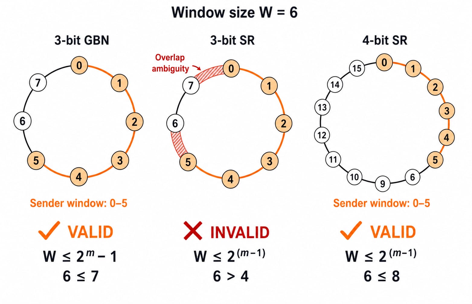
Keep W = 6. In a Go-Back-N-style scheme, an m-bit sequence field permits W <= 2^m - 1. Three bits provide 0 to 7 and a maximum window of 7, so six fits.
Selective Repeat requires W <= 2^(m-1). Three bits permit 4, so W = 6 needs four bits, with a limit of 8. Otherwise, a delayed duplicate could enter the new receive window after wraparound. Half the modulus keeps old and new ranges separate.
Scheme | Sequence bits | Maximum safe | Is |
|---|---|---|---|
Go-Back-N | 3 | 7 | Yes |
Selective Repeat | 3 | 4 | No |
Selective Repeat | 4 | 8 | Yes |
These error-control constraints sit above the flow-control window. Not every sliding-window system uses either ARQ rule.
ACK policy and piggybacking change overhead
Here, ACK 3 confirms frames through 3, moving the lower window edge beyond them. Some texts label the next frame expected. Either convention works, but do not mix them.
Let a standalone ACK contain 80 bits. At 2 Mb/s, serialisation takes 80/(2 x 10^6) = 0.00004 s = 40 microseconds. If the receiver completes frame 0 at 14 ms, has reverse data ready at 16 ms, and uses a 3 ms delayed-ACK timer, it can attach ACK 0 at 16 ms. If reverse data is not ready by 17 ms, it sends the standalone ACK.
Piggybacking saves a control transmission when reverse data arrives soon. Excessive delay stalls the window. The ACK still acknowledges data and advances the window.
A fixed solving order prevents common errors
Use the same order for timing, throughput, minimum-window, receiver-credit, trace, sequence-bit and piggybacking problems:
Convert bytes to bits.
Compute transmission delay.
Draw last-bit arrival and ACK return times.
Identify the active window limit.
Cap utilisation at
1.Check whether the sequence-number constraint makes that window legal.
Check against T_t = 4 ms, a = 2.5, full-pipe W = 6, and Stop-and-Wait U = 1/6. Using propagation once gives a false cycle. Five propagation-product frames omit the frame being transmitted. W = 6 does not mean six sequence bits. The Go-Back-N limit is unsafe for Selective Repeat. A full receiver buffer signals flow control, not congestion.
About 10 live practice questions combine these Data Link Layer flow-control concepts. For the protocol overview and a fuller ARQ comparison, use Flow Control in the Data Link Layer: Worked Examples. The Selective Repeat ARQ worked example follows per-frame buffering and loss recovery after one frame is lost. Receiver credit and piggyback timing add a separate flow-control layer to the same window arithmetic. Apply the method on Computer Networks MCQs.
Data Link Layer flow-control essentials
One outstanding frame means Stop-and-Wait. Several mean a sliding window. Here, 1 + 2a is the full-pipe threshold, receiver credit may lower it, and sequence space must keep the window unambiguous.
Halve the frame to 500 bytes = 4,000 bits, keeping R = 2 Mb/s and T_p = 10 ms. Now T_t = 4,000/(2 x 10^6) = 2 ms, a = 10/2 = 5, and Stop-and-Wait utilisation is 2/(2+20) = 1/11 = 9.09%. The full-pipe window is 1 + 2(5) = 11. Smaller frames require more frames in flight because propagation is unchanged.
For structured Computer Networks study beyond this numerical, continue with GATE Guidance by Sanchit Sir.
Keep learning

Flow Control in the Data Link Layer: Stop-and-Wait, Sliding Window, and Worked Examples
See Stop-and-Wait, sliding windows, Go-Back-N, and Selective Repeat as parts of one system. One link carries every calculation from efficiency to sequence bits.
Updated 9 Aug 20266 min read93 viewsComputer Networks

Ethernet Cross-Concept MCQs: 12 Solved Data Link Layer Questions
Solve 12 Ethernet questions spanning devices, MAC structure, CSMA/CD, STP, VLANs, collision domains, switch port accounting and frame payload conversion.
Updated 30 Aug 20267 min readComputer Networks MCQs

Pipelining Cross-Concept Problems: CPI, Hazards and Cache Stalls
Build one reliable cycle ledger for a five-stage pipeline, then use it to combine load-use stalls, branch penalties and cache misses without mixing units.
Updated 3 Nov 20265 min readComputer Organization & Architecture

Multi-Topic General Hindi for Teaching Exams: Cross-Concept Notes and Worked Set
Learn to separate meaning, word formation, usage, and comprehension when one Hindi passage supports several question types. Then practise the method on a fully solved set.
Updated 4 Aug 20266 min readCTET & UPTET