

Single-Source Shortest Path (SSSP) Algorithms Compared: Worked Example and Exam Traps
Choose the right SSSP algorithm by tracing one six-vertex graph with BFS, DAG relaxation, Dijkstra and Bellman-Ford, then test the common traps.
KnowledgeGate Team
Exam prep & CS education
Updated 13 Nov 20266 min read

Knowing the names BFS, Dijkstra and Bellman-Ford is not enough. The real decision is whether the graph is weighted, contains a negative edge, is acyclic, or asks for all pairs rather than one source. A familiar algorithm on the wrong graph can still produce a plausible but incorrect answer. That distinction matters in GATE CS preparation and in implementation. Dijkstra becomes invalid when a negative edge can improve a vertex that has already been finalised.
Single-source shortest paths: define the problem before choosing an algorithm
For a graph G=(V,E) with edge weight w(u,v) and one source S, the SSSP problem finds the minimum total edge weight from S to every reachable vertex. Initialise d[S]=0; an unreachable vertex keeps distance infinity. Minimum total weight does not necessarily mean minimum number of edges.
Do not mix three scopes. A single-pair query asks only for S to T. SSSP asks for S to every vertex. All-pairs shortest paths asks for every ordered source-destination pair. One SSSP run can answer a single-pair query, while Floyd-Warshall solves the larger all-pairs problem.
The earlier Shortest Path Algorithms: Dijkstra, Bellman-Ford and Floyd-Warshall guide traces each major method on a separate example. Here, one fixed graph isolates how unit weights, acyclicity, negative edges and source scope change the SSSP choice. Relaxation supplies the common operation: if d[u] + w(u,v) < d[v], update d[v] and parent[v].
SSSP algorithms compared: BFS, DAG relaxation, Dijkstra and Bellman-Ford
Method | Correct input condition | Negative edges | Reachable negative cycle | Core idea | Standard time |
|---|---|---|---|---|---|
BFS | Unweighted graph or every edge has the same unit cost | Not a weighted-SSSP method | Not applicable to its intended model | Queue by hop level |
|
DAG shortest path | Weighted directed acyclic graph | Allowed | Impossible in a DAG | Relax once in topological order |
|
Dijkstra | All reachable edge weights are non-negative | Not allowed | Outside its precondition | Finalise the smallest tentative distance greedily |
|
Bellman-Ford | General directed weighted graph | Allowed | Detects one reachable from the source | Repeated edge relaxation |
|
Choose in that order. Unit weights imply BFS. A known DAG permits one topological pass even with negative edges. Otherwise, Dijkstra needs all relevant edges to be non-negative; Bellman-Ford handles possible negative edges or reachable negative-cycle detection.
Fully worked example: run one six-vertex graph four ways
Use vertices {S,A,B,C,D,T}, source S, and directed edges S->A(2), S->B(5), A->C(2), A->D(7), B->C(-6), B->D(4), C->D(2), C->T(5), D->T(1). The edge B->C=-6 is the only negative edge, and the graph has no cycle.
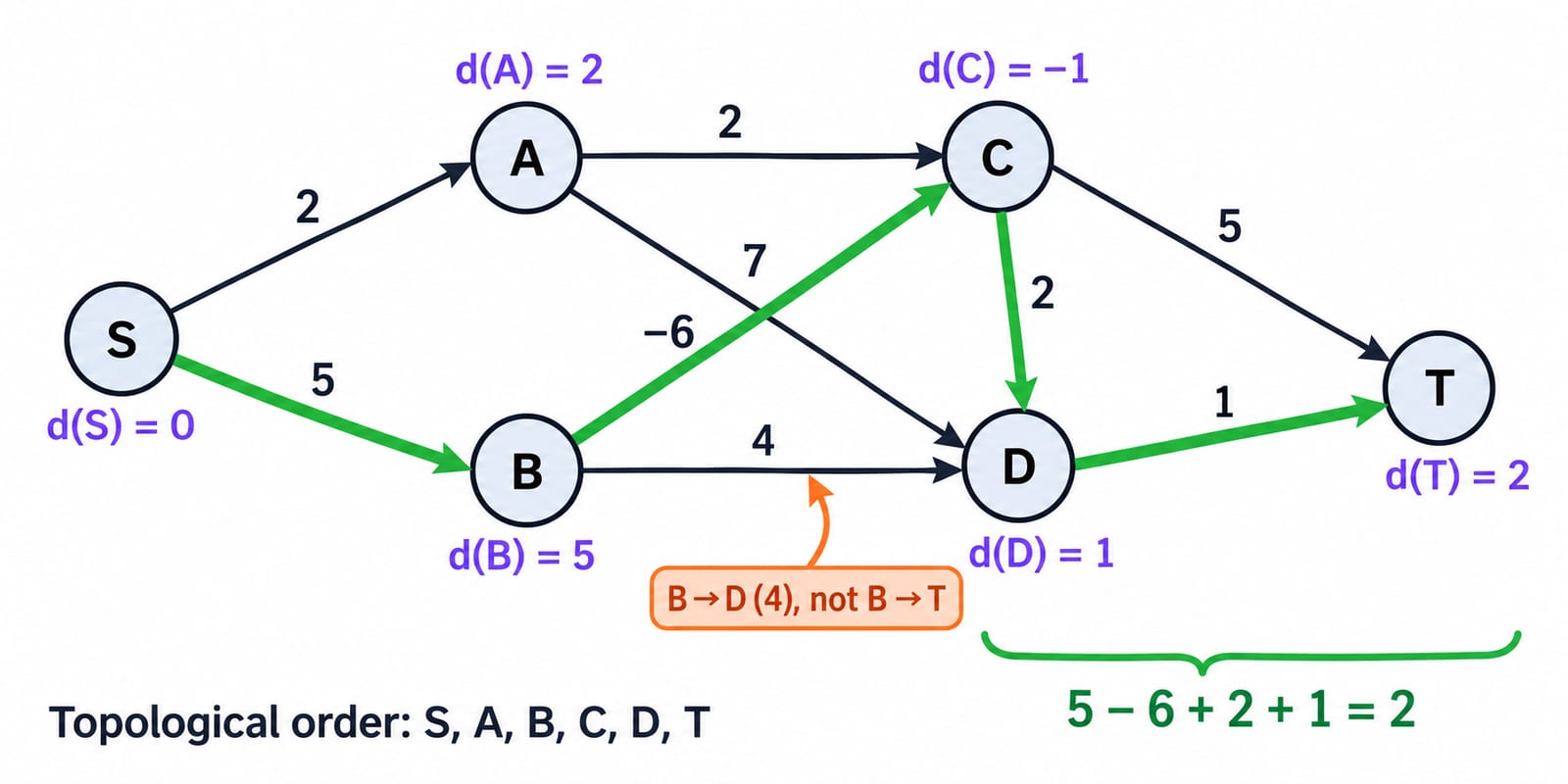
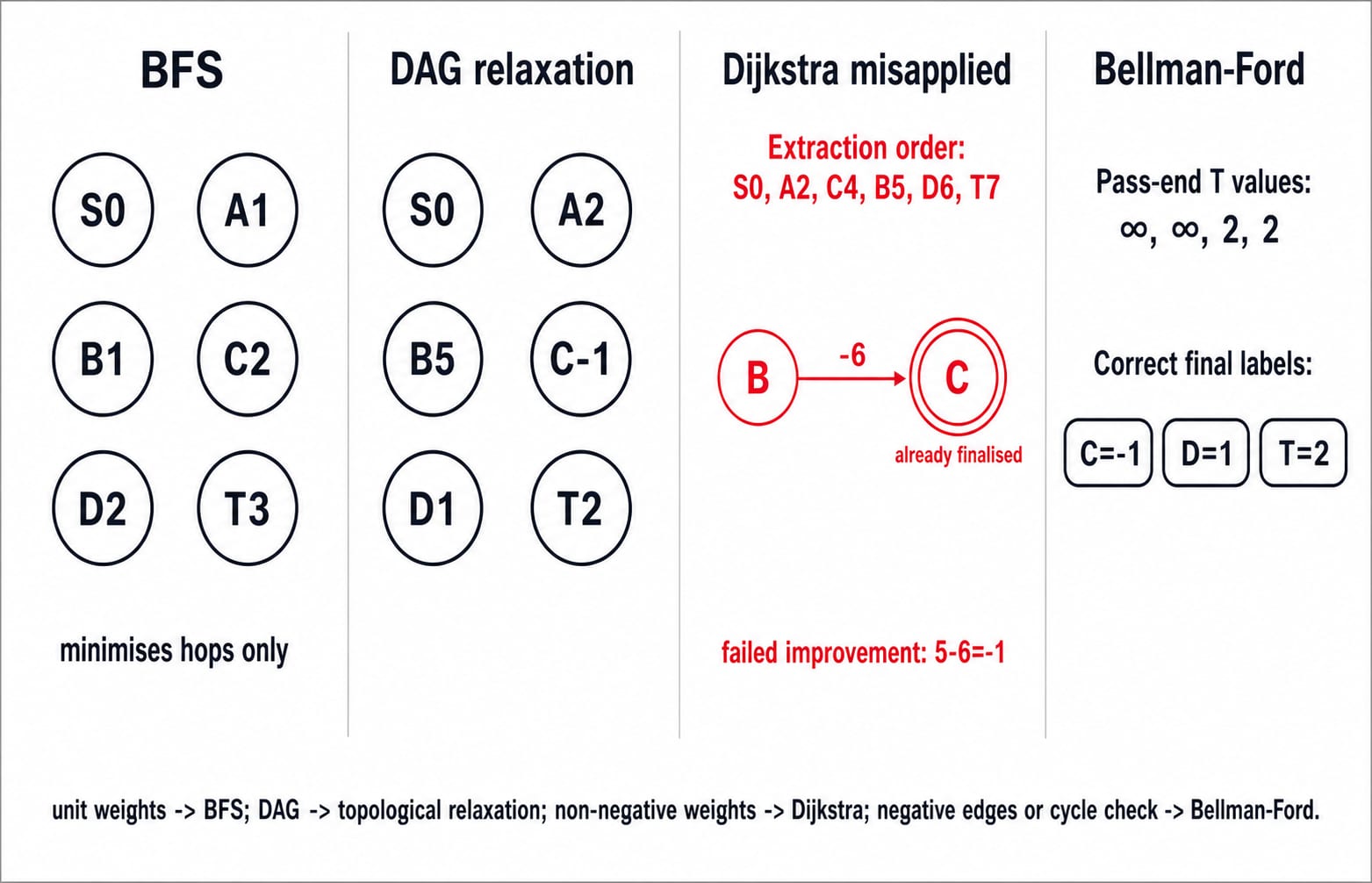
For DAG relaxation, take topological order S,A,B,C,D,T. Processing S gives A=2, B=5. Processing A gives C=4, D=9. Processing B improves C from 4 to 5+(-6)=-1, while D stays 9. Processing C gives D=min(9,-1+2)=1 and T=-1+5=4. Processing D improves T to 1+1=2.
The final distances are d(S)=0, d(A)=2, d(B)=5, d(C)=-1, d(D)=1, d(T)=2. The shortest S to T path is S->B->C->D->T, with weight 5-6+2+1=2.
For Bellman-Ford, scan edges in this deliberately awkward order: C->D, D->T, C->T, A->C, A->D, S->A, B->C, B->D, S->B.
Stage | S | A | B | C | D | T |
|---|---|---|---|---|---|---|
Initial | 0 | infinity | infinity | infinity | infinity | infinity |
After pass 1 | 0 | 2 | 5 | infinity | infinity | infinity |
After pass 2 | 0 | 2 | 5 | -1 | 9 | infinity |
After pass 3 | 0 | 2 | 5 | -1 | 1 | 2 |
After pass 4 | 0 | 2 | 5 | -1 | 1 | 2 |
Pass 4 makes no update, so early stopping is safe. To reconstruct the path, follow parents as T<-D<-C<-B<-S; distance labels alone do not identify the route.
The same graph separates hop count from Dijkstra's weight precondition
Ignore the numerical weights for a moment. With outgoing neighbours processed alphabetically, BFS produces hop levels S:0, A:1, B:1, C:2, D:2, T:3. It correctly minimises hops in an unweighted interpretation. Its three-edge route is not evidence of minimum weighted cost, because the true weight-2 route uses four edges.
Now misapply Dijkstra. The extraction order is S(0), A(2), C(4), B(5), D(6), T(7). When B is extracted, B->C=-6 would improve C from 4 to 5-6=-1, but C has already been finalised. The wrong labels are C=4, D=6, T=7. This does not refute Dijkstra. It violates Dijkstra's non-negative-edge precondition.
Change only B->C from -6 to +6. Dijkstra is now valid, and all weighted methods return C=4, D=6, T=7.
Why the guarantees differ, plus the all-pairs boundary
BFS processes paths by increasing edge count. DAG relaxation works because predecessors precede successors. In Dijkstra's algorithm, once every edge weight is non-negative, the smallest tentative label cannot be improved by a later edge, so extracting it as final is provably safe. After pass i, Bellman-Ford has found every shortest path using at most i edges. That is why V-1 passes suffice when no reachable negative cycle exists, since a simple shortest path uses at most V-1 edges.
Floyd-Warshall handles negative edges and computes all pairs in O(V^3) time and O(V^2) space. A route through a negative cycle has no finite minimum. Do not choose it for a one-source request.
High-value SSSP mix traps: edge shifts, negative cycles and parents
Adding the same constant to every edge can change the shortest path. Direct edge S->T=5 loses to S->X=2 and X->T=2, total 4. Add 2 per edge: the direct route becomes 7, while the two-edge route becomes 4+4=8, so the winner switches. Multiplying every edge by the same positive constant preserves path ordering; adding per edge favours fewer-edge paths.
Return to the main graph and add only D->B(3). The reachable cycle B->C->D->B has weight -6+2+3=-1. Use the earlier scan order, followed by D->B. After the five required passes, labels include B=3, C=-2, D=0, T=1. On the extra scan, B->C lowers C from -2 to -3, proving a reachable negative cycle. Vertices on or reachable from that cycle have no finite shortest distance.
Two habits close out the remaining traps. Never relax an edge whose tail vertex is still at distance infinity, and update parent[v] only when a strict distance improvement occurs. Keep the two records straight: the distance array gives the costs, while the parent chain gives the actual route.
How exam-style questions test SSSP comparisons
Exam questions ask you to choose from the input conditions, trace a stated pass or extraction order, test an edge transformation, or identify a reachable negative cycle.
Try these against the worked graph:
After B is processed in the DAG pass, what is d(C)? The answer is d(C)=-1, since 5 + (-6) = -1.
After Bellman-Ford pass 2 in the given edge order, what is d(D)? The answer is d(D)=9.
Why can Dijkstra not finalise C first here? Because the negative edge B->C has not yet been examined, so C's label can still fall.
Use the GATE Test Series for timed Algorithms practice.
The short version and the next step
Use this decision checklist:
Identify unit or weighted edges.
Check whether the graph is a DAG.
Scan for negative weights.
Decide one source versus all pairs.
Decide whether negative-cycle detection is required.
BFS is for unit weights, DAG relaxation for an acyclic weighted graph, Dijkstra for non-negative weights, and Bellman-Ford for negative edges or cycle detection.
Redraw the graph and reproduce both tables without looking. Then change B->C to +6 and predict every final label. Continue with structured GATE Algorithms preparation.
Go deeper with the full courseAlgorithms
Keep learning
Shortest Path Algorithms: Dijkstra, Bellman-Ford and Floyd-Warshall with Worked Examples for GATE CS
Learn the relaxation idea behind shortest paths, trace three core algorithms by hand, and choose the right method from edge weights and source count.
Updated 21 Sep 20265 min read56 viewsDSA & Algorithms

Graph Algorithms: BFS, DFS, and shortest paths worked out
Graph algorithms explained: adjacency matrix vs list, BFS and DFS traversal order, edge classification, topological sort, and Dijkstra shortest paths.
Updated 30 Oct 20265 min read65 viewsDSA & Algorithms

Sorting Algorithms Compared: complexity, stability, and the n log n lower bound
Sorting algorithms compared: bubble, insertion, selection, merge, quick and heap sort with best, average and worst time, stability, and the n log n bound.
Updated 30 Oct 20266 min read350 viewsDSA & Algorithms

Encapsulation MCQs: 12 Solved OOP Questions with Explanations
Practise 12 real encapsulation questions and learn how to separate bundling, data hiding, abstraction, security, and the main OOP pillars.
Updated 30 Oct 20267 min readMCQ Practice