

Selection Sort Explained: Step-by-Step Trace, Complexity and Exam Traps
Learn the invariant behind Selection Sort, trace every pass, derive its exact comparison count, and avoid common stability and swap-count traps.
KnowledgeGate Team
Exam prep & CS education
Updated 18 Nov 20265 min read

Selection sort seems simple, but exams rarely stop at its definition. They ask for the array after a named pass, exact comparison and exchange counts, and whether equal records retain their order. In the standard minimum-selection, swap-based version, each pass finds the minimum in the unsorted suffix and swaps it into the next position.
Selection sort fixes one final position in every pass
Before pass i, using zero-based indexing, A[0..i-1] is the sorted prefix containing the i smallest keys in their final positions. A[i..n-1] is the unsorted suffix. Find its minimum, store the index, and exchange it with A[i] only if the indices differ.
for i = 0 to n - 2
    minIndex = i
    for j = i + 1 to n - 1
        if A[j] < A[minIndex]
            minIndex = j
    if minIndex != i
        swap A[i], A[minIndex]
After fixing the first n-1 positions, the final element is necessarily correct. Ascending selection sort chooses the minimum for the left boundary; the descending version chooses the maximum. Sorting sits inside the wider algorithms syllabus covered in GATE CS Exam Preparation.
The invariant also proves correctness. Before the first pass, the empty prefix is trivially final. Assume positions 0 through i-1 contain the i smallest keys in order. The minimum of the remaining suffix is therefore the next smallest key; swapping it into A[i] extends the final prefix without disturbing earlier positions. When i reaches n-2, only one suffix value remains, so the whole array is sorted. The suffix may still be in any order during an earlier pass, and nearly sorted input does not shorten its scan.
Selection sort worked example: trace all four passes
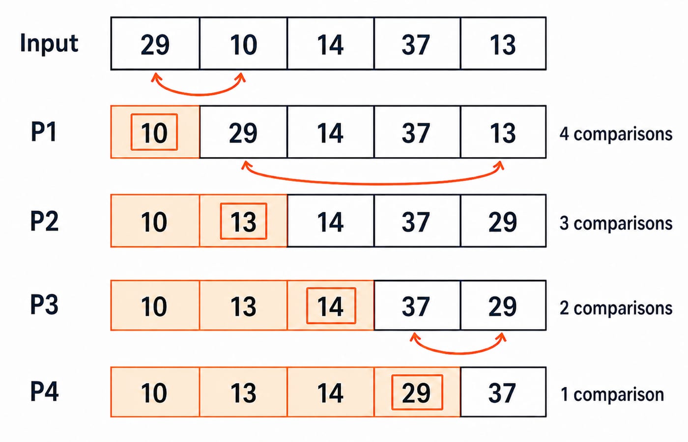
Take A=[29,10,14,37,13]. Keep values and indices distinct: in pass 2, the minimum is value 13 at current index 4.
Pass | Unsorted suffix | Selected minimum | Swap | Array after pass | Comparisons |
|---|---|---|---|---|---|
1 |
|
|
|
| 4 |
2 |
|
|
|
| 3 |
3 |
|
| None |
| 2 |
4 |
|
|
|
| 1 |
The totals are 4+3+2+1=10 key comparisons and 3 actual exchanges because the pass-3 self-swap is skipped. After pass k, the first k cells are final, not merely sorted relative to one another.
Selection sort complexity comes from a fixed comparison sum
Successive suffix scans make n-1,n-2,...,1 comparisons, so
(n-1)+(n-2)+...+1 = n(n-1)/2.
For n=5, this is 5x4/2=10; for n=100, it is 100x99/2=4,950. Even sorted input needs every scan, so best, average and worst time are Theta(n^2). Selection sort is non-adaptive, in-place and uses Theta(1) auxiliary space.
Comparisons are not exchanges. [1,2,3,4,5] needs 10 comparisons and 0 exchanges. [2,3,4,5,1] also needs 10 comparisons but exactly 4 exchanges. Conditional-swap selection sort makes at most n-1 exchanges. If pseudocode performs an unconditional self-swap, the question's convention changes the reported count.
Count conventions must come from the pseudocode. Key comparisons count evaluations of A[j] < A[minIndex]; loop-bound checks and the minIndex != i test are not key comparisons. An exchange may be reported as one swap or as three assignments through a temporary variable. The five-element trace therefore has 10 key comparisons, 3 swaps and, under the three-assignment convention, 9 data assignments caused by swaps. Naming the convention prevents a correct trace from receiving the wrong operation count.
Selection sort is in-place but not stable
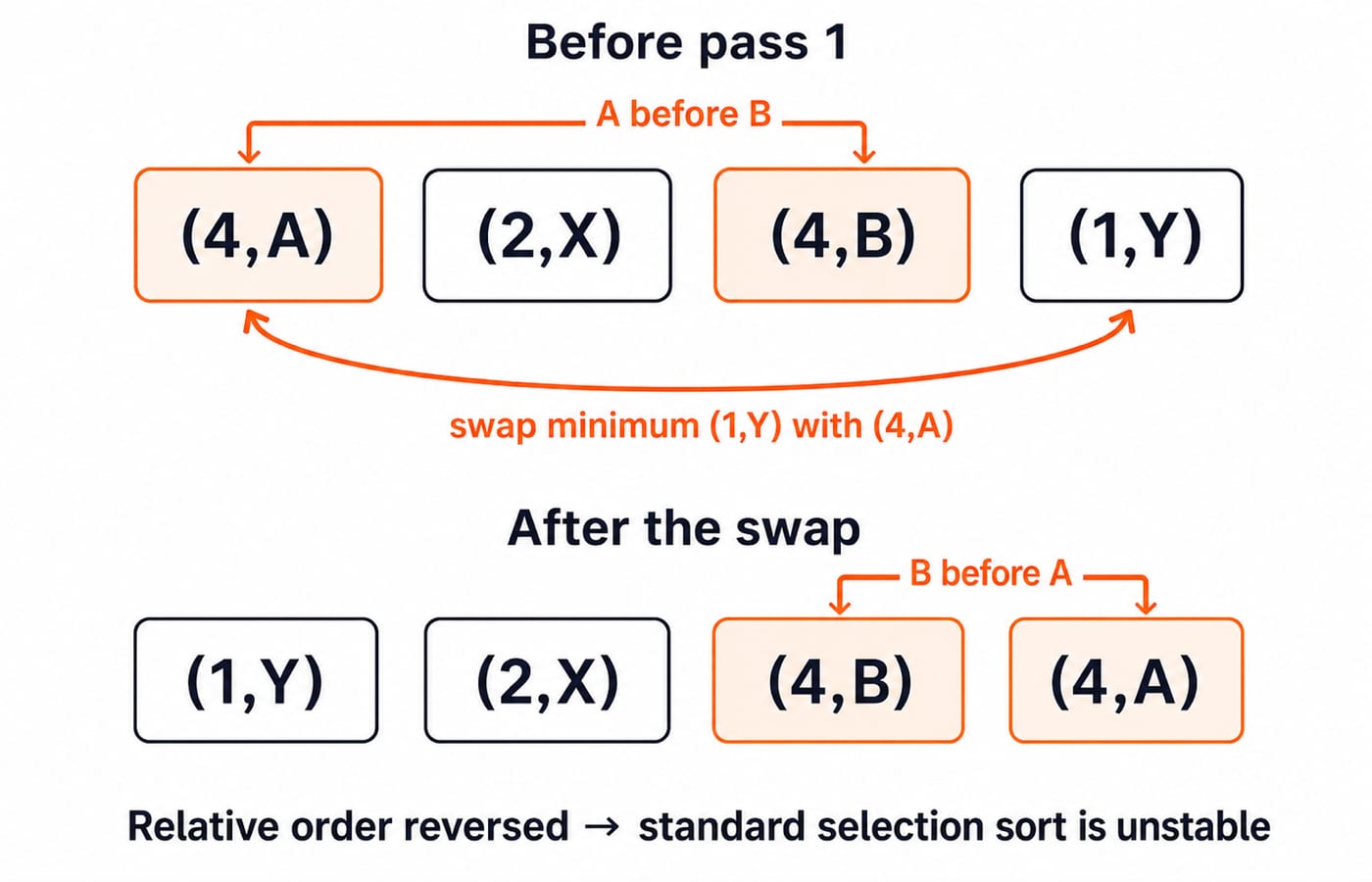
Stability means equal-key records retain their original relative order. Consider [(4,A),(2,X),(4,B),(1,Y)], where record A precedes record B among the key-4 entries. Pass 1 swaps (1,Y) with (4,A), producing [(1,Y),(2,X),(4,B),(4,A)]. Now B precedes A, proving that standard swap-based selection sort is unstable.
Using < rather than <= to select the first minimum does not repair this example. The long-distance swap causes the reversal. A stable variant can remove the minimum and shift intervening records one position right, but that may require linear data movement per pass and loses the standard version's low-exchange advantage.
Selection sort versus bubble sort and insertion sort
Algorithm | Best time | Worst time | Stable | Adaptive | In-place | Data movement |
|---|---|---|---|---|---|---|
Selection |
|
| No | No | Yes | At most |
Optimised bubble |
|
| Yes | Yes | Yes | Up to quadratic swaps |
Insertion |
|
| Yes | Yes | Yes | Up to quadratic shifts |
Selection sort is rarely chosen for large inputs, but its at-most n-1 exchanges can matter when writes are substantially more expensive than reads. Insertion sort gains a linear best case from stopping within its sorted prefix; optimised bubble sort gains one from a no-swap pass. Selection sort gains neither because it scans every remaining suffix. For a cross-family decision by stability, space and growth rate, use Sorting Algorithms: Complexity, Stability, n log n Bound. Selection sort's decisive properties are its fixed comparison count, bounded exchanges and unstable long-distance swap.
Each pass makes a locally final choice and never revisits the fixed prefix. This connects to Greedy Algorithms: Strategy and Problems, although selection sort's exam identity remains its trace, comparison cost and stability.
Selection sort exam traps: trace, count and classify
Use these keyed checks:
After
kpasses, the firstkkeys are final.Comparisons equal
n(n-1)/2, notn-1.Actual exchanges are at most
n-1, not quadratic.Standard selection sort is in-place but unstable.
Descending order selects the maximum; it does not keep selecting the minimum while merely scanning backwards.
Trace A=[64,25,12,22,11]. Pass 1 selects 11 and gives [11,25,12,22,64]. Pass 2 selects 12 and gives [11,12,25,22,64]. The suffix need not be sorted, so [11,12,22,25,64] is not the state after two passes.
Before each practice trace, identify the loop variant, then record the suffix minimum, array state, cumulative key comparisons and actual exchanges after every pass. The GATE Test Series is an optional route for mixed timed practice.
Selection sort in the short version and the next step
Select the smallest suffix key.
Place it at the left boundary.
Repeat for
n-1passes.Comparisons are always
n(n-1)/2.Exchanges are at most
n-1.The standard algorithm is in-place, non-adaptive and unstable.
Thus, [29,10,14,37,13] becomes [10,13,14,29,37] with 10 comparisons and 3 actual exchanges. Use GATE Guidance by Sanchit Sir if you want this topic placed inside a structured Algorithms sequence.
Self-test: What is the array after two passes, and how many total comparisons are required, when sorting [7,4,9,2,6,1]?
Answer: Pass 1 gives [1,4,9,2,6,7]; pass 2 gives [1,2,9,4,6,7]; total comparisons are 6x5/2=15.
Go deeper with the full courseAlgorithms
Keep learning

Coding Questions for GATE CS: Trace Outputs and Complexity Step by Step
Learn a reliable way to solve coding output and complexity questions. Three fully traced C examples cover loops, mutation, recursion and operation counts.
Updated 29 Aug 20265 min readC Programming & Data Structures
Radix Sort and Counting Sort: Worked Examples, Complexity and Exam Traps
See how counting sort builds cumulative positions and how LSD radix sort depends on stable digit passes. Two traced examples turn formulas and exam traps into checks you can reproduce.
Updated 17 Nov 20265 min readDSA & Algorithms
Merge Sort Interview Questions and Answers: Traces, Complexity, and Code
Prepare crisp merge sort interview answers through a fully traced array, boundary-safe Java implementation, complexity proof, stability example, and inversion-count follow-up.
Updated 3 Nov 20266 min readInterview Corner
Heap Sort Interview Questions and Answers: Trace, Code, and Follow-Ups
Learn to build a max-heap, trace every extraction, explain iterative sift-down, justify the time and space bounds, and handle common Heap Sort follow-ups.
Updated 2 Nov 20265 min readInterview Corner