

Approximation Algorithms Explained: Ratios, Vertex Cover and a Worked 2-Approximation
Learn what an approximation guarantee means, how ratios differ for minimisation and maximisation, and why a simple Vertex Cover algorithm has a tight factor of 2.
KnowledgeGate Team
Exam prep & CS education
Updated 29 Oct 20265 min read
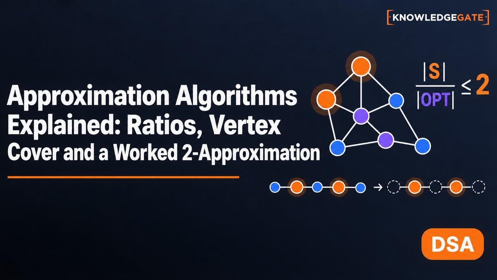
You may understand greedy algorithms yet still wonder what separates an approximation algorithm from a plausible heuristic. The difference is not that one always looks cleverer on a sample input. It is a proved guarantee that holds across all valid inputs. A correct analysis reads approximation ratios in the right direction, traces an unweighted Vertex Cover algorithm on a concrete graph, and derives why its factor is 2.
What an approximation algorithm guarantees
An optimisation problem defines feasible solutions and an objective to minimise or maximise. For instance I, let OPT(I) be the best feasible objective value and A(I) the value returned by polynomial-time algorithm A.
An approximation algorithm returns a feasible solution and has a proved bound relating A(I) to OPT(I). A heuristic can work well without that worst-case guarantee. This quality guarantee is separate from runtime and one observed result.
Approximation helps when exact optimisation is difficult at scale. Yet NP-hardness neither proves P != NP nor automatically supplies a useful approximation. The GATE CS Exam Preparation category places these ideas beside the surrounding algorithms sequence.
Approximation ratios for minimisation and maximisation
For a minimisation problem, an alpha-approximation satisfies A(I) <= alpha * OPT(I) for every valid input, where alpha >= 1. If OPT = 8 and A = 12, the observed ratio is A/OPT = 12/8 = 1.5. This run satisfies a factor-2 bound because 12 <= 2 * 8 = 16.
For a maximisation problem with positive objective values, the direction reverses: A(I) >= OPT(I)/alpha. Equivalently, OPT(I)/A(I) <= alpha. If OPT = 120 and A = 80, then OPT/A = 120/80 = 1.5, or A = (2/3)OPT. Do not reuse A/OPT blindly for maximisation.
Both calculations describe observed performance, not a worst-case proof. Suppose a proved 2-approximation returns A = 9 when OPT = 8. Its observed ratio is 9/8 = 1.125, but its certified guarantee remains 2 until a stronger proof establishes a smaller bound for every input.
The main approximation patterns to recognise
Problem | Construction | Guarantee | Condition |
|---|---|---|---|
Unweighted Vertex Cover | Take both endpoints of maximal-matching edges | Factor | Undirected, unweighted graph |
Metric TSP | Double an MST, form an Euler tour, shortcut repeats | At most | Triangle inequality |
Set Cover | Greedily cover the most remaining elements |
| Universe has |
0/1 Knapsack FPTAS | Scale values, run a reduced dynamic program | At least | Chosen |
For example, H_4 = 1 + 1/2 + 1/3 + 1/4 = 25/12, about 2.083. This interprets the notation, not the proof.
A PTAS is polynomial in input size for each fixed epsilon. An FPTAS is polynomial in both input size and 1/epsilon. Revise graph language with Graph Theory: Euler, Hamiltonian and Coloring before the example.
The unweighted Vertex Cover 2-approximation algorithm
For undirected graph G = (V,E), a vertex cover is a set C subseteq V containing at least one endpoint of every edge. The objective is a minimum-size cover, not merely a feasible one.
Start with C_cover = empty and M = empty. While an uncovered edge remains, choose one, (u,v). Add it to M, add u and v to C_cover, then delete every edge incident to either endpoint. Return C_cover when no edge remains.
The selected edges form a maximal matching because none can be added at the end. A maximum matching is unnecessary. Arbitrary choices may change the cover, but not the factor-2 proof.
Worked example: the algorithm reaches its factor-2 bound
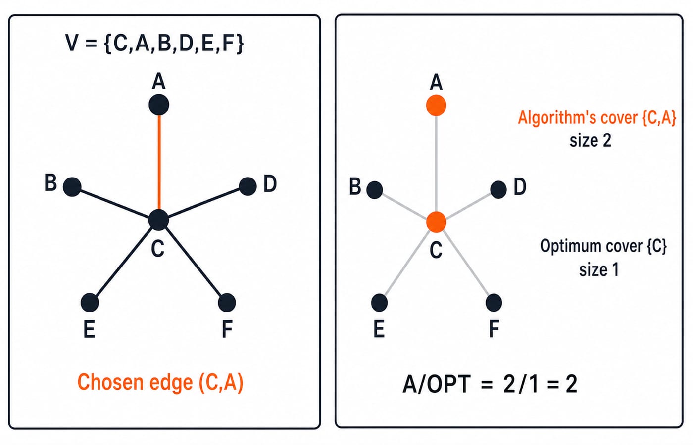
Use the star V = {C,A,B,D,E,F} with E = {(C,A),(C,B),(C,D),(C,E),(C,F)}. Its centre is C and its leaves are A, B, D, E, and F. Choose (C,A) first.
Step | Matching | Cover | Edges remaining |
|---|---|---|---|
Initial |
|
| All 5 edges |
Choose |
|
| All edges incident to |
Stop |
|
|
|
Deleting incident edges removes all five edges, so the loop stops. The cover is feasible because every original edge contains centre C, which is in C_cover.
Now compute the optimum. The empty set covers nothing, while the one-vertex set {C} covers all five edges. Therefore OPT = 1. The algorithm returns A = |{C,A}| = 2, so A/OPT = 2/1 = 2. The analysis is tight on this instance, although the output exceeds the optimum by only one vertex.
Why the proof gives a factor of 2
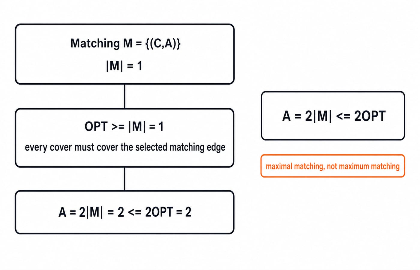
First, M is a matching. After choosing an edge, the algorithm deletes every edge incident to its endpoints. A later chosen edge therefore cannot share either endpoint.
Second, every vertex cover must take one endpoint of each edge in M. These edges are vertex-disjoint, so that requires at least |M| distinct vertices. Thus OPT >= |M|.
The algorithm takes both endpoints, so A = 2|M|. Therefore:
A = 2|M| <= 2OPT.
On the star, M = {(C,A)}, |M| = 1, and OPT >= 1. The result A = 2|M| = 2 gives 2 <= 2OPT = 2. Feasibility proves the result is a cover, while the matching lower-bounds the unknown optimum. Maximal means no edge can be added. Maximum means largest cardinality.
How exams and interviews test approximation algorithms
Typical tasks ask you to compute a ratio, apply a stated factor, trace this Vertex Cover algorithm, or explain why |M| lower-bounds OPT. Other tasks distinguish maximal from maximum matching, test the triangle-inequality condition for double-tree TSP, or compare PTAS with FPTAS.
The archived official GATE 2026 CS syllabus from IIT Guwahati places greedy, dynamic programming, divide-and-conquer, graph traversals, minimum spanning trees, and shortest paths under Algorithms, but does not name Approximation Algorithms separately. Topic inclusion can change between cycles, so use the official syllabus for the cycle you are preparing for.
For adjacent graph practice, use Graph MCQs: BFS, DFS and Connectivity; for broader timed practice, use the GATE Test Series.
Common traps, the short version and next step
Six traps to correct: approximation is not heuristic without a proved bound; minimisation and maximisation ratios face opposite ways; feasibility is not a quality proof; one good run does not improve the guarantee; maximal matching is not necessarily maximum; metric TSP bounds need the triangle inequality.
The four-line method is:
State the objective and
OPT.Write the correct ratio direction.
Find a lower bound for minimisation or upper bound for maximisation.
Compare the feasible result with that bound.
Memory hook: M = 1, A = 2, OPT = 1, ratio 2. Cover the proof, then reconstruct A = 2|M| <= 2OPT from the star. Continue with GATE Guidance by Sanchit Sir for the broader sequence.
Keep learning
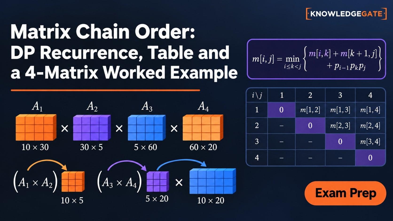
Matrix Chain Order: DP Recurrence, Table and a 4-Matrix Worked Example
See why order changes scalar cost even when the final matrix does not. Build both DP tables for p = [5, 10, 3, 12, 5] and recover the 405-cost solution.
Updated 10 Nov 20266 min readDSA & Algorithms
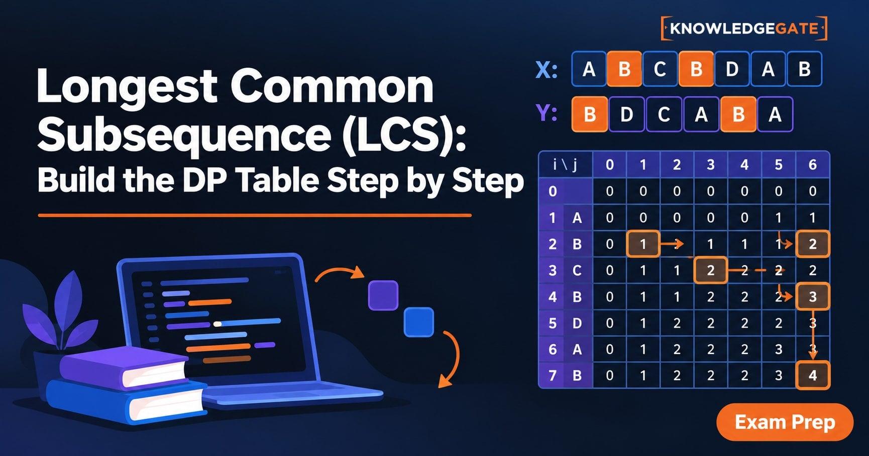
Longest Common Subsequence (LCS): Build the DP Table Step by Step
Build an LCS table from its prefix state, trace every important cell, and backtrack one valid answer. The worked example ends with GTAB.
Updated 9 Nov 20265 min readDSA & Algorithms
Fractional Knapsack Explained: Greedy Logic, Worked Example and Exam Traps
Learn why ratio order is optimal for divisible items, trace every step of a capacity-50 solution, and avoid common greedy and arithmetic mistakes.
Updated 8 Nov 20266 min readDSA & Algorithms
Growth Rate Comparisons: How to Order Functions Step by Step
Learn how to normalise and order logarithmic, polynomial, exponential, and factorial functions without letting a small-value table mislead you.
Updated 6 Nov 20265 min readDSA & Algorithms