

Branch and Bound Explained: Bounds, Pruning and Worked Examples
Learn how Branch and Bound chooses live nodes and proves optimality. Follow a best-bound knapsack trace and a smaller assignment-cost example step by step.
KnowledgeGate Team
Exam prep & CS education
Updated 30 Oct 20266 min read
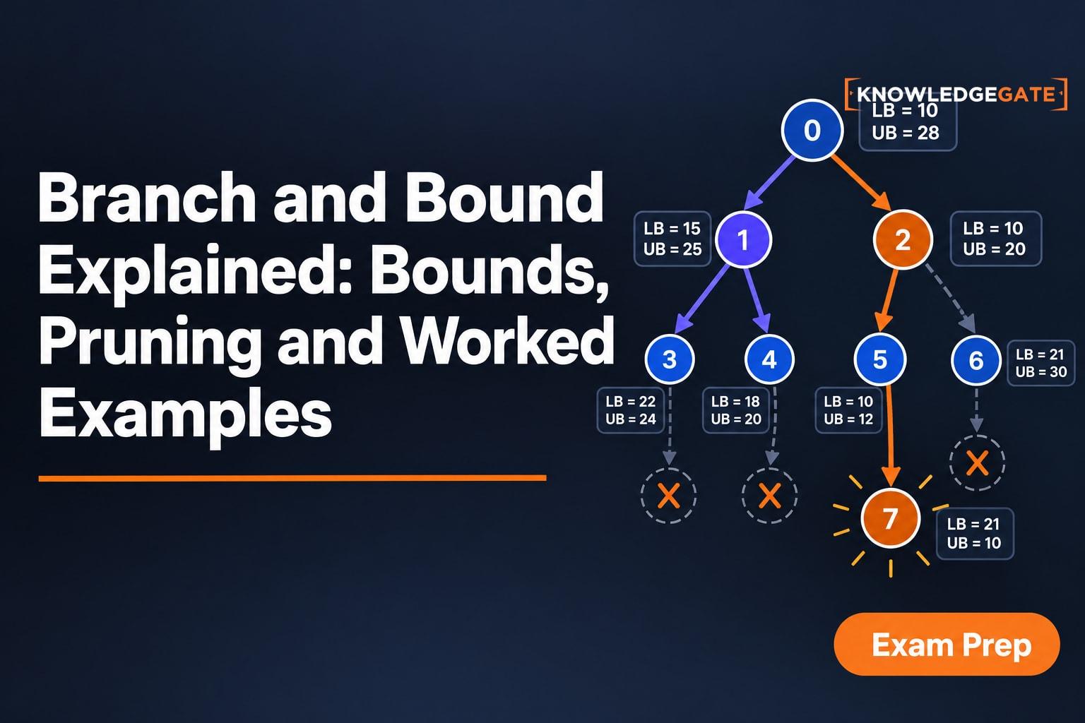
Branch and Bound is often reduced to a tree with a few crossed-out nodes. The real difficulty is knowing what a bound promises, which live node is expanded next, and why pruning cannot discard a better answer. A valid bound must not exclude a better completion, node selection determines which live node expands next, and pruning must preserve every better answer. Minimisation reverses the direction: a three-worker assignment trace uses a lower bound and prunes costs that cannot improve the incumbent.
Branch and Bound From Zero: The Search Model
Branch and Bound is an exact optimisation framework over a state-space tree. Branching fixes decisions. A bound estimates the best objective that any completion below a partial node could achieve. The incumbent is the best complete feasible solution found so far.
A live node may still be expanded. The live node currently being expanded is the E-node. A node becomes dead when it is infeasible, fully explored, or safely pruned.
For maximisation, use an upper bound UB and prune when UB <= incumbent profit. For minimisation, use a lower bound LB and prune when LB >= incumbent cost. These equality rules apply when only one optimal value or solution is needed. If every optimal solution must be listed, an equality-bound node may still contain another optimum.
How Bounds and Node Selection Work
The control strategy selects the next E-node. FIFO uses queue order; LIFO uses the newest live node. Best-bound uses a priority queue, selecting the largest UB for maximisation or the smallest LB for minimisation. With valid bounds and stopping, order affects efficiency, not correctness.
A bound may be optimistic and unattainable, but must never exclude a better completion. Tighter valid bounds often prune more but may cost more to compute. In 0/1 knapsack, a fractional item is allowed only while calculating UB. Every real solution still chooses either 0 or 1 of each item.
The loop is simple: remove the most promising live node, branch, reject infeasible children, update the incumbent, compute bounds, and keep only children that can beat it. The state-space tree models decisions, not necessarily a binary-tree data structure.
Worked 0/1 Knapsack Setup and the Fractional Upper Bound
Let capacity W = 16. Sort the items by profit-to-weight ratio:
Item | Weight | Profit | Ratio |
|---|---|---|---|
A | 2 | 40 | 20 |
B | 5 | 30 | 6 |
C | 10 | 50 | 5 |
D | 5 | 10 | 2 |
Branch A, B, C, D; 1 includes and 0 excludes. Reject a child if its weight exceeds 16.
First build a feasible incumbent. Take A and B, skip C because it does not fit, then take D. Its weight is 2 + 5 + 5 = 12, and its profit is 40 + 30 + 10 = 80. This starts the search, not a proof of optimality.
For the root's fractional bound, take all of A and B. The remaining capacity is 16 - 7 = 9, so the relaxation takes 9/10 of C:
UB(root) = 40 + 30 + (9/10 × 50) = 115.
At A = 0, take B and C, then 1/5 of D:
UB(A = 0) = 30 + 50 + (1/5 × 10) = 82.
These bounds describe possibilities, not feasible 0/1 profits.
Best-Bound Search Trace, Pruning and Optimality
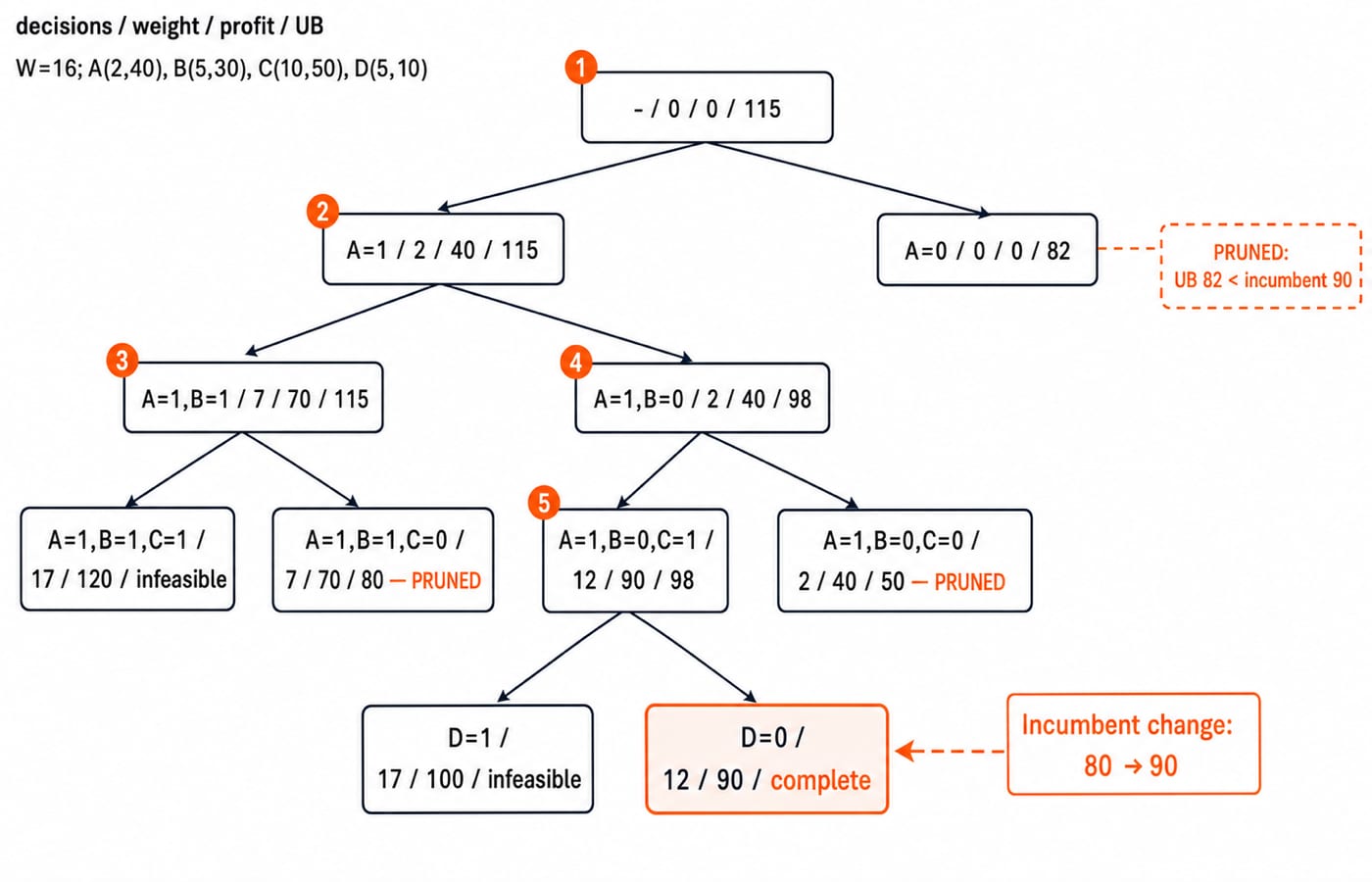
Start with incumbent profit 80. The priority queue always pops the largest UB.
Popped node | Weight | Profit | UB | Children kept | Reason |
|---|---|---|---|---|---|
root | 0 | 0 | 115 |
| Both bounds exceed 80 |
| 2 | 40 | 115 |
| Both bounds exceed 80 |
| 7 | 70 | 115 | none |
|
| 2 | 40 | 98 |
|
|
| 12 | 90 | 98 | none |
|
The bound 98 at A=1,B=0 is 40 + 50 + (4/5 × 10). Its C=1 child is feasible with profit 90 if undecided items are treated as excluded, so the incumbent becomes 90. After expanding that child, every remaining live bound is at most 82 and cannot beat 90.
The chosen solution is A + C. Its weight check is 2 + 10 = 12 <= 16, and its profit is 40 + 50 = 90. Feasibility supplies a candidate. Pruning every node that might have beaten it supplies the proof of optimality.
A Minimisation Example: Three-Worker Assignment
Each worker must receive one different job. The costs are:
Worker | J1 | J2 | J3 |
|---|---|---|---|
W1 | 9 | 2 | 7 |
W2 | 6 | 4 | 3 |
W3 | 5 | 8 | 1 |
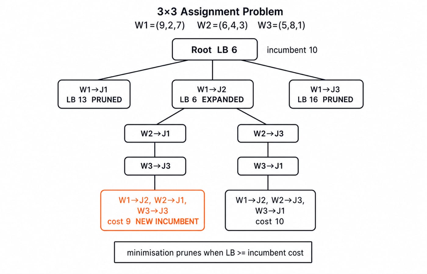
The root row-minimum lower bound is 2 + 3 + 1 = 6. It is unattainable because W2 and W3 both prefer J3. Start with assignment (W1-J2, W2-J3, W3-J1), costing 2 + 3 + 5 = 10.
Branch on W1. The bounds are W1-J1: 9 + 3 + 1 = 13, W1-J2: 2 + 3 + 1 = 6, and W1-J3: 7 + 4 + 5 = 16. Prune 13 and 16 against incumbent 10. Under W1-J2, choosing W2-J1 forces W3-J3, giving 2 + 6 + 1 = 9. The alternative gives 2 + 3 + 5 = 10. The minimum cost is 9. The related graph-optimisation vocabulary is covered in Graph Theory.
Correctness, Complexity and What Branch and Bound Is Not
The correctness argument has three parts. Every solution lies below a decision path. Every pruned subtree has a valid bound that cannot beat the incumbent. When no live node can beat it, the incumbent is optimal.
The worst case remains expensive. Binary include-or-exclude search may examine O(2^n) nodes, and best-bound memory can also grow exponentially. Bounding improves practical search, not worst-case complexity.
Backtracking mainly cuts infeasible branches. Branch and Bound also cuts feasible-looking branches through objective bounds. Greedy commits locally without reopening alternatives. Dynamic programming reuses overlapping subproblems when a suitable recurrence exists. Exhaustive search lacks objective-bound pruning. Real algorithms may combine these ideas, so the distinctions describe decision logic, not mutually exclusive software labels.
How Exams and Interviews Can Test Branch and Bound
Useful question shapes include computing a fractional UB, choosing the next E-node under FIFO, LIFO or best-bound order, pruning after an incumbent update, reversing the minimisation inequality, completing a partial tree, separating relaxation values from feasible objectives, and spotting an invalid bound.
Check the anchor values: knapsack root UB 115, optimum profit 90, assignment root LB 6, and optimum cost 9. Always confirm the current syllabus and paper instructions on your exam board's official site.
Once the method feels solid, the GATE Test Series is available for timed practice.
Branch and Bound Proof Checklist and Next Practice
Before crossing out a node, ask four questions. Is its bound valid for every completion? Is the bound direction correct for maximisation or minimisation? Has a complete feasible incumbent been recorded? Does the pruning inequality actually rule out improvement? If any answer is no, the prune is unsafe. Equality can be discarded only when one optimum is enough.
Hide both figures and reconstruct the queue, bounds, incumbent updates and prunes from the raw tables. Then use GATE Guidance by Sanchit Sir for the broader Algorithms sequence.
Keep learning
Matrix Chain Order: DP Recurrence, Table and a 4-Matrix Worked Example
See why order changes scalar cost even when the final matrix does not. Build both DP tables for p = [5, 10, 3, 12, 5] and recover the 405-cost solution.
Updated 10 Nov 20266 min readDSA & Algorithms
Longest Common Subsequence (LCS): Build the DP Table Step by Step
Build an LCS table from its prefix state, trace every important cell, and backtrack one valid answer. The worked example ends with GTAB.
Updated 9 Nov 20265 min readDSA & Algorithms
Fractional Knapsack Explained: Greedy Logic, Worked Example and Exam Traps
Learn why ratio order is optimal for divisible items, trace every step of a capacity-50 solution, and avoid common greedy and arithmetic mistakes.
Updated 8 Nov 20266 min readDSA & Algorithms
Growth Rate Comparisons: How to Order Functions Step by Step
Learn how to normalise and order logarithmic, polynomial, exponential, and factorial functions without letting a small-value table mislead you.
Updated 6 Nov 20265 min readDSA & Algorithms