

Algebraic Computation: Polynomial Multiplication, DFT and Strassen's Algorithm
Learn how representation cuts arithmetic work through one exact convolution, a four-point DFT pipeline, and a fully checked Strassen matrix product.
KnowledgeGate Team
Exam prep & CS education
Updated 28 Oct 20265 min read
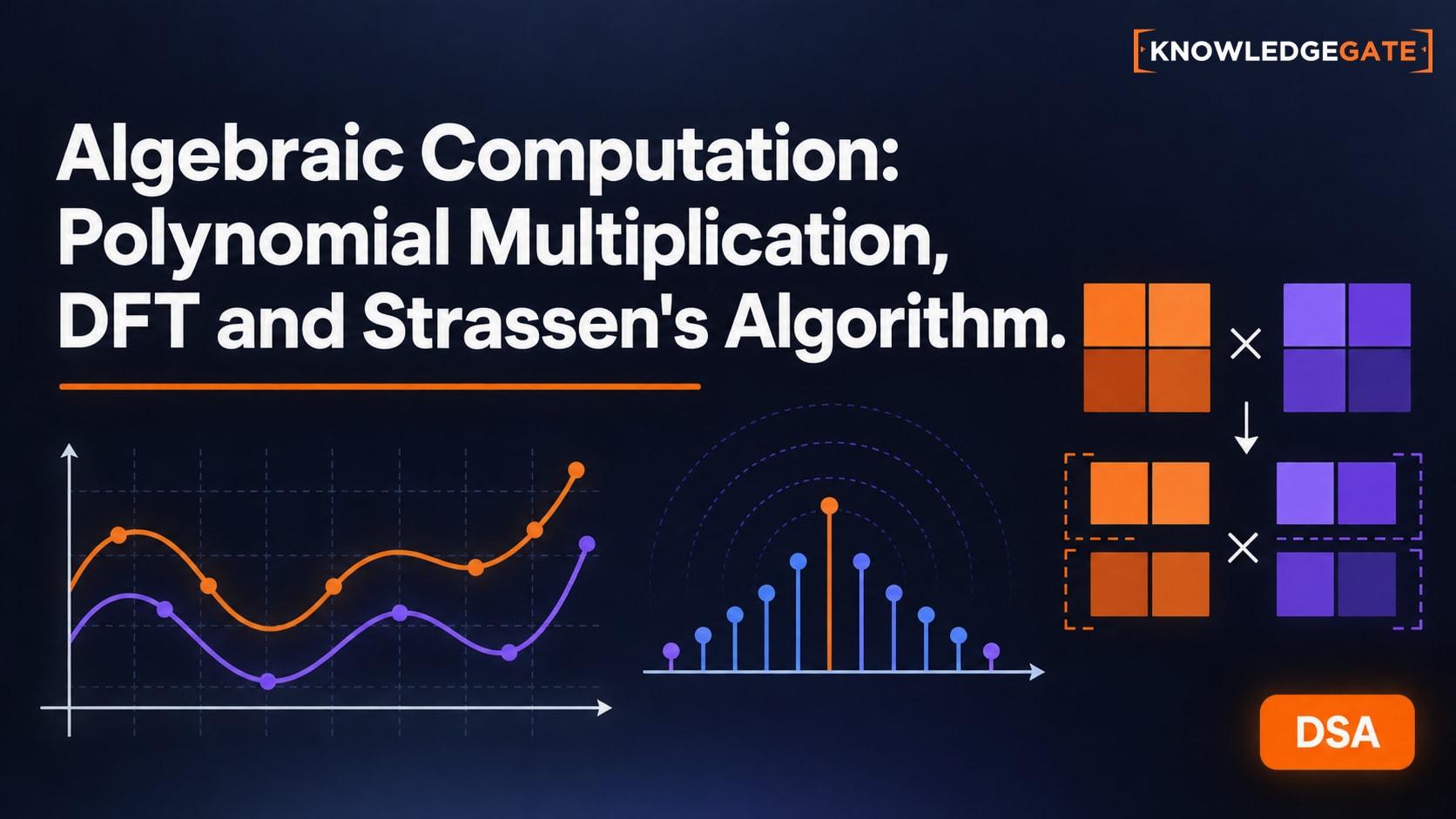
Polynomial coefficients, a DFT matrix and Strassen formulas can look like three unrelated sets of facts. The common idea is that algebraic computation represents objects so a costly operation can be replaced by fewer, better-structured arithmetic operations. An exact polynomial product can be computed directly or through a four-point DFT, and a Strassen matrix multiplication can be checked by the ordinary method.
Algebraic Computation Means Exploiting Structure
Algebraic computation is the design and analysis of algorithms that operate on algebraic objects such as numbers, polynomials, vectors and matrices. Its objective is to obtain the same exact result with fewer or better-organised arithmetic operations by exploiting structure, representation or divide-and-conquer.
This is broader than symbolic manipulation. Multiplying polynomials, evaluating a DFT and multiplying numeric matrix arrays are all algebraic computations. It is also distinct from learning the axioms of algebraic structures. Group Theory: Groups, Rings and Fields for GATE CS covers that adjacent foundation; algebraic computation instead studies algorithms over algebraic objects.
Applications include polynomial arithmetic, matrix computation, graphics transformations, linear recurrences, coding calculations and signal transforms. Not all use Strassen or the FFT.
Representation and Cost Models Come Before the Algorithm
Take A(x) = 1 + 2x + 3x^2. Its coefficient vector is [1,2,3]. At x = 2, its value is:
A(2) = 1 + 2(2) + 3(2^2) = 1 + 4 + 12 = 17.
Coefficient form exposes convolution; values at selected points make multiplication pointwise. Only the representation changes.
Take A = [[1,2],[3,4]]. In a 2 x 2 example, each block is a scalar. In an n x n divide-and-conquer algorithm, the four blocks are (n/2) x (n/2) matrices. Write those dimensions before writing a recurrence.
The arithmetic model counts additions, subtractions and multiplications as primitive. Bit complexity also considers operand length: multiplying 2^1000 - 1 need not cost the same as multiplying 7 by 8, though each counts as one multiplication here.
Baseline Worked Example: Polynomial Multiplication by Convolution
Multiply A(x) = 1 + 2x + 3x^2 by B(x) = 4 + 5x. The result has degree 2 + 1 = 3, so it needs four coefficients, c0 through c3.
c0 = 1(4) = 4c1 = 1(5) + 2(4) = 5 + 8 = 13c2 = 2(5) + 3(4) = 10 + 12 = 22c3 = 3(5) = 15
Therefore:
C(x) = 4 + 13x + 22x^2 + 15x^3
Its coefficient vector is [4,13,22,15]. This product forms six coefficient products and performs two non-trivial sums. It is wrong to call the four output coefficients four operations. In general, direct convolution of two length-n coefficient arrays takes quadratic arithmetic work. Also remember that a degree-three polynomial has four coefficients.
The Four-Point DFT Turns Convolution into Pointwise Products
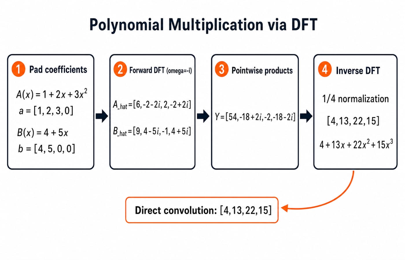
The inputs have lengths three and two, so their product needs 3 + 2 - 1 = 4 coefficients. Zero-pad them to a = [1,2,3,0] and b = [4,5,0,0].
Fix the convention first. Let omega = exp(-2 pi i / 4) = -i. Then:
W4 = [[1,1,1,1], [1,-i,-1,i], [1,-1,1,-1], [1,i,-1,-i]]
Multiplying by this matrix gives:
A_hat = W4 a = [6,-2-2i,2,-2+2i]
B_hat = W4 b = [9,4-5i,-1,4+5i]
Multiply corresponding values:
Y = [54,-18+2i,-2,-18-2i].
The inverse transform uses the conjugate sign and a 1/4 normalisation. For example, its second coefficient is:
(54 + i(-18+2i) - (-2) - i(-18-2i)) / 4 = 52 / 4 = 13.
The full inverse returns [4,13,22,15], exactly the direct-convolution result. Multiplication by a dense DFT matrix is still quadratic. The FFT is the recursive algorithm that evaluates the DFT in Theta(n log n) arithmetic operations, so DFT and FFT are related terms, not synonyms.
Fully Worked Strassen Example with Seven Scalar Multiplications
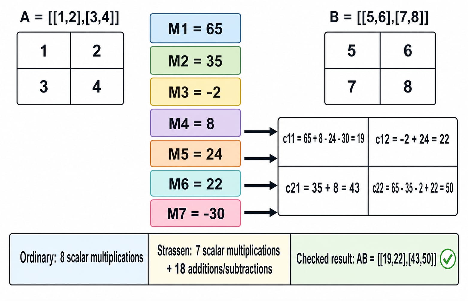
Let A = [[1,2],[3,4]] and B = [[5,6],[7,8]], with entries a=1, b=2, c=3, d=4, e=5, f=6, g=7, and h=8.
Record the ordinary product for checking:
AB = [[1(5)+2(7),1(6)+2(8)],[3(5)+4(7),3(6)+4(8)]] = [[19,22],[43,50]].
Now use one fixed Strassen convention:
M1 = (a+d)(e+h) = 5(13) = 65M2 = (c+d)e = 7(5) = 35M3 = a(f-h) = 1(-2) = -2M4 = d(g-e) = 4(2) = 8M5 = (a+b)h = 3(8) = 24M6 = (c-a)(e+f) = 2(11) = 22M7 = (b-d)(g+h) = (-2)(15) = -30
Recombine them without changing conventions:
c11 = M1+M4-M5+M7 = 65+8-24-30 = 19c12 = M3+M5 = -2+24 = 22c21 = M2+M4 = 35+8 = 43c22 = M1-M2+M3+M6 = 65-35-2+22 = 50
Both methods give [[19,22],[43,50]]. Ordinary 2 x 2 multiplication uses eight scalar multiplications and four additions. This Strassen convention uses seven multiplications plus 18 additions or subtractions, including the operand combinations and output recombinations. Its advantage appears through recursion on large matrices, not through fewer total primitive operations in this tiny example.
Derive the Complexity Instead of Memorising the Exponent
Classical block matrix multiplication makes eight recursive products:
T(n) = 8T(n/2) + Theta(n^2) = Theta(n^3).
Strassen makes seven recursive products and spends quadratic work combining blocks:
T(n) = 7T(n/2) + Theta(n^2) = Theta(n^(log_2 7)), where log_2 7 is approximately 2.807.
For length-n polynomial inputs, direct convolution and a dense DFT matrix-vector product are both Theta(n^2). FFT-based multiplication uses two forward transforms, n pointwise products and one inverse, keeping the total at Theta(n log n).
Implementation choices also depend on padding, recursion overhead, cache behaviour and complex-number round-off. No universal input size makes Strassen the best choice. The GATE CS Exam Preparation Courses & Test Series catalogue places these ideas in a broader study plan, while each recurrence follows from the number and size of recursive calls.
How Questions Test Algebraic Computation, and the Traps to Repair
Questions can test the objective, a polynomial-multiplication bound, a 4 x 4 DFT matrix under a stated root, coefficient and point-value forms, or Strassen's saving.
Trap | Consequence | Repair |
|---|---|---|
No zero padding | Circular convolution or lost coefficients | Use at least |
DFT sign not declared | Conjugated matrix or wrong imaginary signs | Write |
Inverse factor omitted | Every recovered coefficient is scaled | Divide by |
Strassen formulas mixed across conventions | Wrong recombination | Keep one formula set |
Seven multiplications means seven operations | Addition overhead ignored | Count additions separately |
Degree | Off-by-one size | Degree |
Practice questions on this topic ask you to reproduce these steps rather than recall a formula, so drill the convolution, the transform and the recombination separately. Use Graph MCQs: 10 Solved BFS, DFS, Connectivity (GATE) for adjacent algorithm practice and the GATE Test Series: Mocks and Topic-wise Tests for broader timed work.
Algebraic Computation: The Short Version and Next Step
Representation controls available operations. Direct coefficient multiplication is convolution. A DFT makes convolution pointwise. Strassen trades one recursive multiplication for extra additions. Declare the DFT convention, then verify the result directly.
Reproduce [4,13,22,15], both DFT value sets, and all seven M values without looking. Explain each recurrence in one sentence. GATE Guidance by Sanchit Sir offers a structured full-subject route. If studying only this topic, redo both methods and repair every sign or size error.
Keep learning
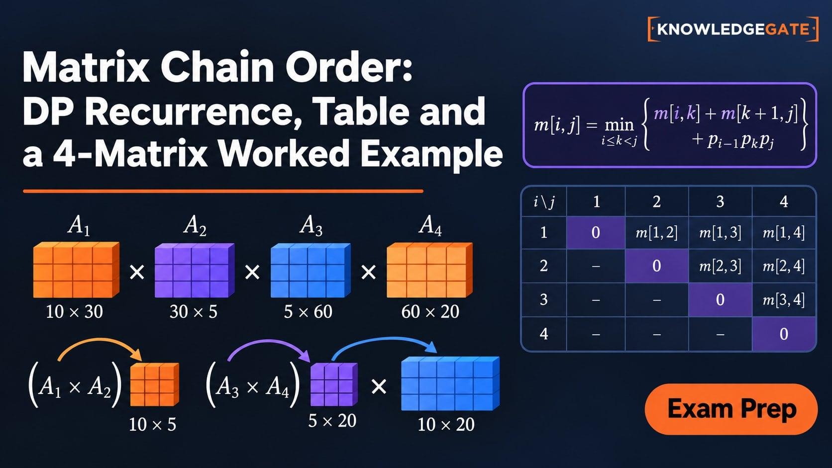
Matrix Chain Order: DP Recurrence, Table and a 4-Matrix Worked Example
See why order changes scalar cost even when the final matrix does not. Build both DP tables for p = [5, 10, 3, 12, 5] and recover the 405-cost solution.
Updated 10 Nov 20266 min readDSA & Algorithms
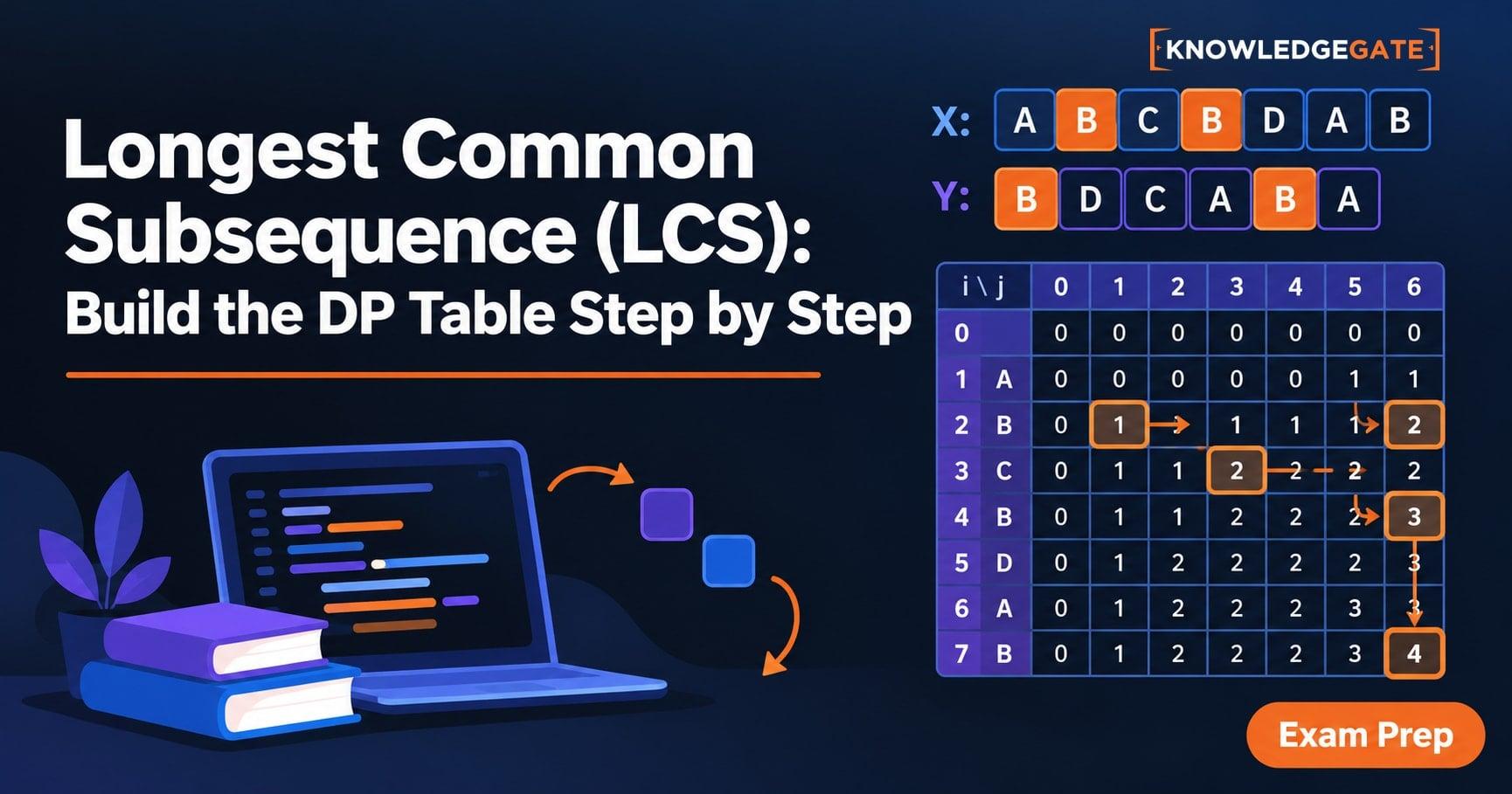
Longest Common Subsequence (LCS): Build the DP Table Step by Step
Build an LCS table from its prefix state, trace every important cell, and backtrack one valid answer. The worked example ends with GTAB.
Updated 9 Nov 20265 min readDSA & Algorithms
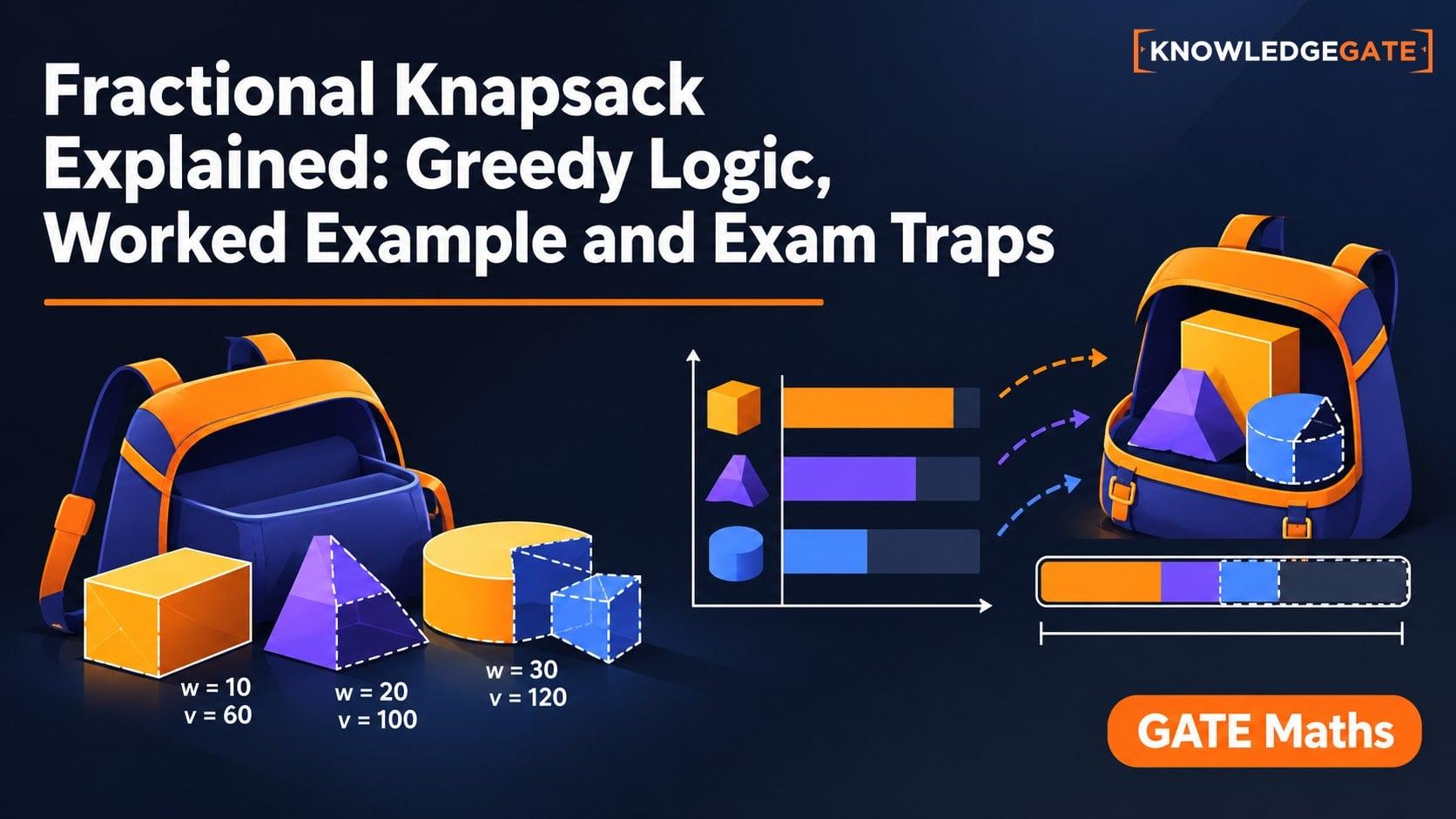
Fractional Knapsack Explained: Greedy Logic, Worked Example and Exam Traps
Learn why ratio order is optimal for divisible items, trace every step of a capacity-50 solution, and avoid common greedy and arithmetic mistakes.
Updated 8 Nov 20266 min readDSA & Algorithms
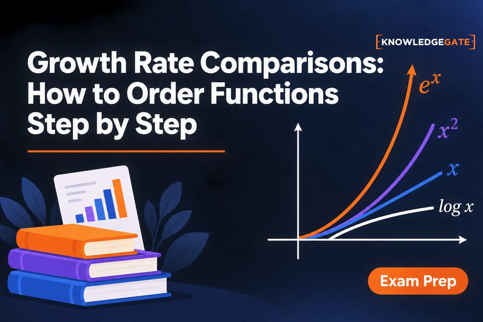
Growth Rate Comparisons: How to Order Functions Step by Step
Learn how to normalise and order logarithmic, polynomial, exponential, and factorial functions without letting a small-value table mislead you.
Updated 6 Nov 20265 min readDSA & Algorithms