

Performance & Speedup in Computer Architecture: Formulas, Worked Examples and GATE Traps
Learn to compare processors fairly, calculate pipeline gains and apply Amdahl's law through step-by-step numericals with unit checks.
KnowledgeGate Team
Exam prep & CS education
Updated 4 Nov 20266 min read

A processor with a higher clock rate is not automatically faster. A pipeline may improve throughput even while one instruction takes longer, and a 25% fall in execution time does not mean a 25% performance gain. Execution time and performance use reciprocal relationships, so each percentage must be calculated from its own denominator.
Performance, execution time, throughput and speedup
Response time, or latency, is the time for one task. Throughput is tasks completed per unit time. For the same workload:
Performance = 1 / execution time
The comparison formula is:
Speedup(new over old) = T_old / T_new = Performance_new / Performance_old
A result above 1 means the new system is faster. If a task falls from 10 to 7.5 seconds, time falls by (10 - 7.5) / 10 = 25%. But speedup is 10 / 7.5 = 1.333, so performance rises by 33.3%.
Reverse it: a 25% performance rise makes time 10 / 1.25 = 8 seconds, a 20% reduction. Time change and performance change use different denominators.
Place this topic within Computer Organization & Architecture. If the terminology feels unfamiliar, revise the wider CS fundamentals first.
The CPU performance equation and a fair machine comparison
For one program and one input:
CPU time = Instruction count × CPI × Clock cycle time
Since Clock cycle time = 1 / Clock rate, the same equation becomes:
CPU time = (Instruction count × CPI) / Clock rate
Clock rate alone cannot decide the faster machine. Instruction count can change with the compiler, while CPI depends on the instruction mix and design. Compare all three for the same workload.
Consider a program that executes 1.2 × 10^9 instructions.
For Machine A, CPI = 2.0 and clock rate is 3 GHz:
T_A = (1.2 × 10^9 instructions × 2.0 cycles/instruction) / (3 × 10^9 cycles/second)
T_A = 2.4 × 10^9 cycles / 3 × 10^9 cycles/second = 0.80 seconds
For Machine B, CPI = 1.5 and clock rate is 2.4 GHz:
T_B = (1.2 × 10^9 × 1.5) / (2.4 × 10^9) = 0.75 seconds
Speedup of B over A is 0.80 / 0.75 = 1.0667, so B's performance is 6.67% higher. Its time is lower by (0.80 - 0.75) / 0.80 = 6.25%. Keep those percentages distinct.
For a dimensional check, instructions cancel with cycles per instruction, then cycles cancel with cycles per second, leaving seconds. Otherwise, the clock-rate term is probably inverted.
What pipelining can and cannot speed up
For a k-stage pipeline processing n independent instructions without stalls:
T_pipeline = (k + n - 1) × t_clk
The pipeline fills, issues one instruction per cycle in steady state, then drains. For the stated non-pipelined implementation, time is n × sum(stage delays).
The pipeline clock is not the average stage delay:
t_clk = maximum stage delay + pipeline-register overhead
The slowest stage controls the clock. Imbalance, register overhead, fill, drain and stalls reduce practical speedup. Approaching k requires large n, balanced stages and negligible overhead. Pipelining in Computer Architecture owns the five-stage mechanics and hazard taxonomy. Here, pipelining is one case in a wider performance comparison that also uses the CPU-time equation and Amdahl's law.
Worked example: a five-stage pipeline for 20 instructions
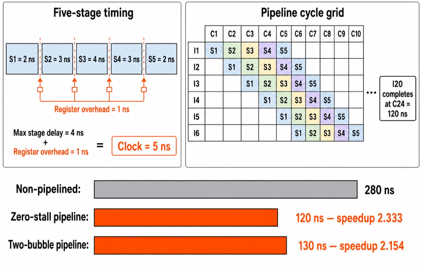
Use the linked pipeline note for stage mechanics and hazard handling. The calculation below compares four performance measures on one workload: batch time, single-instruction latency, throughput and asymptotic speedup. Take stage delays [2, 3, 4, 3, 2] ns, register overhead 1 ns, and n = 20 independent instructions with no stalls.
The non-pipelined time for one instruction is:
2 + 3 + 4 + 3 + 2 = 14 ns
For 20 instructions, T_non-pipeline = 20 × 14 = 280 ns.
The pipeline clock is max(2, 3, 4, 3, 2) + 1 = 4 + 1 = 5 ns. The completion time is:
T_pipeline = (5 + 20 - 1) × 5 = 24 × 5 = 120 ns
So actual speedup is 280 / 120 = 2.333.
The first pipelined instruction has latency 5 × 5 = 25 ns, worse than 14 ns. Yet steady-state throughput is one instruction every 5 ns, or 1 / (5 × 10^-9) = 200 million instructions/second. Pipelining helps the stream, not necessarily one instruction.
For large n, speedup approaches 14 / 5 = 2.8, not 5. Two bubble cycles make time (24 + 2) × 5 = 130 ns and speedup 280 / 130 = 2.154.
Answer template: identify old time, find pipeline clock, count fill plus useful issues plus stalls, match units, then divide old time by new time.
Amdahl's law: why a fast part may give a modest total gain
Amdahl's law measures the total benefit when only part of the original time improves:
Overall speedup = 1 / ((1 - p) + p / s)
Here, p is the affected fraction of original time and s is its speedup. It is not an instruction fraction unless the question says so.
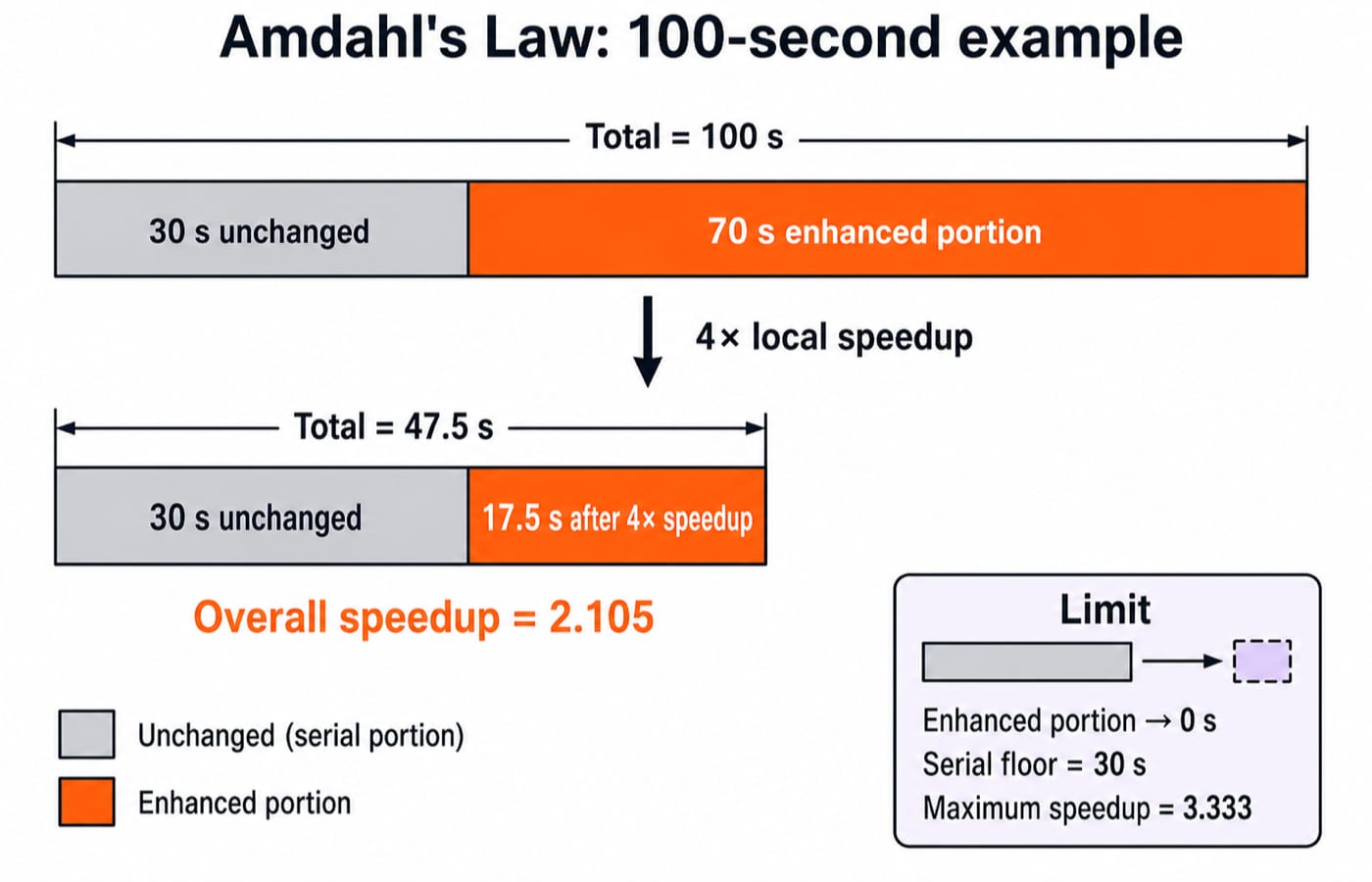
If 70% of original time improves fourfold, normalised new time is:
(1 - 0.70) + 0.70 / 4 = 0.30 + 0.175 = 0.475
Overall speedup is 1 / 0.475 = 2.105. From 100 seconds, the improved part falls from 70 to 70 / 4 = 17.5 seconds; the unchanged 30 seconds makes total time 47.5 seconds.
Infinite speed for the improved part still leaves 30%, so maximum speedup is 1 / 0.30 = 3.333. Multiprocessors in COA: Concepts, Amdahl's Law and Cache Coherence Worked Examples owns processor-count scaling and efficiency. Here, p and s describe any improved component, so the same law also applies to compiler, memory and accelerator changes.
Traps and the ways exam-style questions test speedup
Speedup numericals commonly test the mistakes below. These are exam-style patterns rather than attributed previous-year questions.
Wrong move | Why it fails | Correction |
|---|---|---|
Use | Faster systems then appear to have a value below 1 | Use |
Treat 25% less time as 25% more performance | Time and performance are reciprocals | Recalculate using |
Choose the higher-GHz CPU | CPI and instruction count may differ | Apply the full CPU-time equation |
Use | Instructions overlap | Use |
Ignore register overhead or bubbles | Both increase pipeline time | Include overhead in |
Set speedup equal to stage count | Imbalance, overhead, and finite | Compute both execution times |
Confuse throughput with latency | More completions per second need not shorten one instruction | State which metric changed |
Practise comparing CPUs from instruction count, CPI and clock rate; pipeline time with overhead and bubbles; reverse Amdahl problems; and latency versus throughput.
Reverse checkpoint: with p = 0.75 and overall speedup 2.5, new time is 1 / 2.5 = 0.4. Thus 0.4 = 0.25 + 0.75 / s, then 0.15 = 0.75 / s, so s = 5.
Practise three calculation shapes separately: CPU time from instruction count, CPI and clock rate; pipeline timing with stalls; and Amdahl problems with an unchanged fraction.
The short version and the next problem to solve
Performance is the inverse of execution time.
Speedup is old time divided by new time.
CPU time combines instruction count, CPI and clock rate.
Pipeline time includes fill, drain, register overhead and stalls.
Amdahl's law limits whole-program gain when some work remains unchanged.
Change only n from 20 to 100. Non-pipelined time is 100 × 14 = 1400 ns. Pipeline time is (5 + 100 - 1) × 5 = 520 ns. Speedup is 1400 / 520 = 2.692, moving towards but not beyond the 2.8 limit.
For structured GATE preparation, continue with GATE Guidance by Sanchit Sir. For broader core computer science, use ZERO TO HERO. Always recompute percentages from the time ratio.
Keep learning

Pipelining Basics in Computer Architecture: Clock Cycle, Speedup and Hazard Worked Examples
Learn how to calculate a pipeline clock, fill and drain time, finite-batch speedup, latency, throughput, and the cost of a load-use stall.
Updated 23 Oct 20266 min read106 viewsComputer Organization & Architecture

Pipelining in Computer Architecture: the 5-stage pipeline, speedup, and hazards
Pipelining in computer architecture: the 5-stage pipeline, speedup and throughput formulas, CPI, structural, data and control hazards, and forwarding.
Updated 30 Oct 20265 min read216 viewsComputer Organization & Architecture

Disk Access Time and Performance: Formulas, Worked Example and GATE Traps
Learn how seek time, rotational latency and transfer time combine, then apply the formulas to random and contiguous reads without losing track of units.
Updated 10 Sep 20265 min read284 viewsComputer Organization & Architecture

Performance & Speedup MCQs: 12 Solved Pipelining Questions
Work through 12 solved pipelining questions step by step, from finite pipeline time and latch overhead to bubbles, MIPS, CPI and bottleneck splitting.
Updated 29 Oct 20268 min readComputer Organization MCQs