Natural Language Processing Explained: Pipeline, TF-IDF Worked Example and Exam Patterns
Start from raw text, build BoW and TF-IDF vectors, compute cosine similarity, examine ambiguity, and finish with evaluation and exam-style checks.
KnowledgeGate Team
Exam prep & CS education
Updated 15 Oct 20266 min read
You may recognise chatbots and translation but still be unable to explain what happens between raw text and a model's output. Natural language processing (NLP) is the branch of AI that makes human language computable, but text must first be segmented, represented and interpreted. Natural language processing involves linguistic levels, a pipeline, TF-IDF and cosine calculation, ambiguity, evaluation arithmetic and exam patterns. The Skills category is the broader learning route.
Natural language processing: scope, goals and linguistic levels
NLP uses artificial intelligence and computational linguistics to analyse, represent and generate human language. Human language is productive, contextual and ambiguous, unlike a programming language designed around explicit syntax and semantics. NLP covers far more than chatbots.
Natural language understanding (NLU) maps language to meaning or structure, as in intent classification or information extraction. Natural language generation (NLG) maps a representation or context to language, as in summarisation. Translation, dialogue and question answering can need both.
Level | Question | Example |
|---|---|---|
Morphology | How do word parts combine? |
|
Syntax | How do words form a sentence? | Subject, verb and object |
Semantics | What does it literally mean? | Meaning of a proposition |
Discourse | How do sentences connect? | A pronoun referring to an earlier noun |
Pragmatics | What does the speaker intend here? |
|
The final example is syntactically a question about ability, while pragmatics supplies its normal social purpose.
NLP pipeline: from raw sentence to structured features
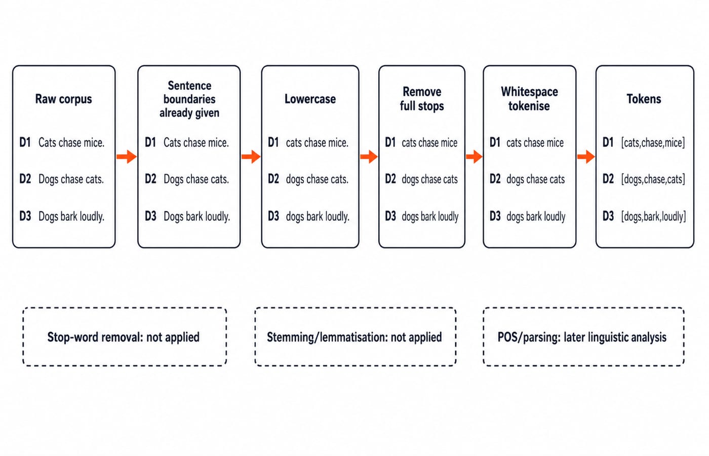
Use one fixed corpus: D1 = "Cats chase mice.", D2 = "Dogs chase cats.", and D3 = "Dogs bark loudly." Sentence boundaries are already given. Lowercase the text, remove the full stops, then split on whitespace. The results are D1=[cats,chase,mice], D2=[dogs,chase,cats], and D3=[dogs,bark,loudly].
Optional stop-word removal may discard useful negation. Stemming can produce a non-word, whereas lemmatisation uses linguistic information to return a dictionary form. Part-of-speech tagging labels roles, parsing captures dependencies or phrases, and named-entity recognition marks people, organisations or places. This corpus needs no stop-word removal, stemming or lemmatisation.
As Lexical Analysis in Compiler Design: Tokens, Patterns and Lexemes explains, both pipelines turn characters into units. Compiler tokens follow a formal language; NLP tokenisation must handle language-specific punctuation, contractions, multiword expressions and ambiguity.
Representing text: one-hot vectors, bags of words, n-grams and embeddings
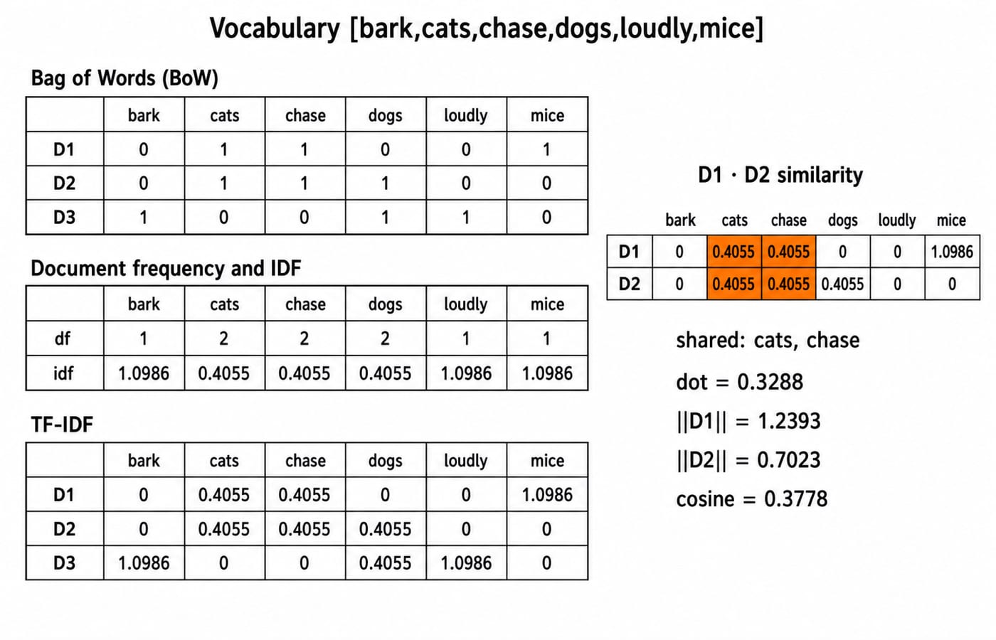
Fix the vocabulary order as [bark,cats,chase,dogs,loudly,mice]. The raw bag-of-words vectors are D1=[0,1,1,0,0,1], D2=[0,1,1,1,0,0], and D3=[1,0,0,1,1,0]. One-hot represents one item; bag-of-words stores document counts but discards order.
N-grams restore limited local order. For dogs chase cats, the unigrams are dogs, chase, cats; the bigrams are dogs chase, chase cats; and the trigram is dogs chase cats. A length L sequence has L-n+1 contiguous n-grams when L>=n, so it has 3-2+1=2 bigrams.
One-hot, bag-of-words and TF-IDF are vocabulary-dependent sparse vectors. Dense embeddings learn continuous, lower-dimensional representations. Contextual embeddings can represent bank differently in river bank and bank loan. Transformers use attention to relate tokens.
Worked TF-IDF example and cosine similarity
Use raw-count TF(t,d)=count(t,d) and unsmoothed IDF(t)=ln(N/df(t)), with N=3. In the fixed vocabulary order, document frequency is [1,2,2,2,1,1]. The IDF row is [ln 3,ln(3/2),ln(3/2),ln(3/2),ln 3,ln 3], approximately [1.0986,0.4055,0.4055,0.4055,1.0986,1.0986].
Multiplying counts by IDF gives:
TF-IDF(D1)=[0,0.4055,0.4055,0,0,1.0986]TF-IDF(D2)=[0,0.4055,0.4055,0.4055,0,0]TF-IDF(D3)=[1.0986,0,0,0.4055,1.0986,0]
mice receives more weight than cats in D1 because it occurs in one document, while cats occurs in two.
Now compare D1 and D2. Their dot product is 0.4055^2+0.4055^2=0.3288. Their norms are ||D1||=sqrt(0.4055^2+0.4055^2+1.0986^2)=1.2393 and ||D2||=sqrt(3x0.4055^2)=0.7023. Therefore cos(D1,D2)=0.3288/(1.2393x0.7023)=0.3288/0.8703=0.3778. This measures positive lexical overlap through cats and chase; it does not prove identical meaning.
Why NLP is hard: ambiguity, context and variation
Ambiguity | Example | Competing readings |
|---|---|---|
Lexical |
| Financial institution or river edge |
Syntactic |
| The telescope modifies |
Semantic or scope |
| One shared book or possibly different books |
Pragmatic |
| A statement or an indirect request to close a window |
dog bites man and man bites dog have identical bag-of-words counts but opposite roles. In Maya gave Riya the notes because she had copied them, resolving she needs wider context and may remain genuinely ambiguous.
Spelling variants, code-mixed text, morphology, named entities, jargon and unseen words affect systems. Preprocessing does not erase them. Language models learn statistical patterns, not guaranteed truth or speaker intent, so fluent output can still be wrong.
NLP approaches, tasks and evaluation with actual values
Rule-based systems use lexicons, grammars and hand-written patterns. Statistical machine learning estimates patterns from labelled or unlabelled data. Neural models learn layered representations, with transformers using attention between tokens. Practical systems can combine approaches; newer does not make every older method useless.
Match evaluation to the output. Sentiment analysis produces a class; named-entity recognition produces labelled spans; part-of-speech tagging produces a label per token; translation and summarisation produce sequences; information retrieval ranks documents; and question answering returns a span or generated response.
For binary sentiment on 40 sentences, let TP=18, FP=3, FN=2, and TN=17.
Accuracy
=(18+17)/40=35/40=0.875.Precision
=18/(18+3)=18/21=0.8571.Recall
=18/(18+2)=18/20=0.9000.F1
=2(0.8571)(0.9000)/(0.8571+0.9000)=0.8780.
Accuracy alone can hide class imbalance. Generated sequences also need different evaluation methods, so no single metric fits every NLP task.
Natural language processing traps and question patterns
Trap | Why it fails | Correction |
|---|---|---|
NLP equals speech recognition | NLP also covers written language | Treat speech as one input or output route |
Tokenisation always splits spaces | Punctuation, contractions and multiword units complicate boundaries | Follow the stated tokenizer |
Stemming equals lemmatisation | Their methods and outputs differ | Check whether linguistic analysis returns a lemma |
Bag-of-words preserves order | It stores counts | Use n-grams or sequence models for order |
Common words always get high TF-IDF | High document frequency lowers IDF | Apply the formula as stated |
Cosine is a distance or truth score | It is a similarity between vectors | Interpret overlap within the representation |
Fluent output proves perfect intent understanding | Fluency can coexist with error | Evaluate against task evidence |
Typical questions ask you to match linguistic levels to examples, trace preprocessing, count n-grams, form a BoW vector in a given order, calculate df, IDF, TF-IDF or cosine similarity, identify ambiguity, or derive precision, recall and F1. Preserve the formula and logarithm base stated in the question.
Check yourself: D2 has 2 bigrams; df(chase)=2; IDF(mice)=ln 3=1.0986; D1/D2 cosine is about 0.3778; sentiment recall is 18/20=0.90. For bigram probabilities and Laplace smoothing, work through Natural Language Processing in AI: Core Concepts, a Worked Bigram Example, and How Exams Test It. Use the six-term corpus above for bag-of-words, TF-IDF, cosine similarity and evaluation arithmetic.
Natural language processing: the short version and next step
Remember the chain: segment and normalise raw language, add linguistic analysis, represent tokens as features, map features to a task output, then evaluate with a task-appropriate measure. The anchors are a six-term vocabulary, IDF 1.0986 for one-document terms, IDF 0.4055 for two-document terms, D1/D2 cosine 0.3778, and sentiment F1 0.8780.
Reproduce the three BoW rows, derive document frequencies, recompute the cosine unaided, then explain why dog bites man and man bites dog defeat bag-of-words. For a structured wider-CS route whose curriculum includes NLP, use Zero to Hero, Complete CS Course. For broader applied AI and machine learning, use AI & ML for Placements.
Keep learning
Foundations and Evolution of AI: Approaches, Timeline and a Worked Rational-Agent Example
Build a connected map of AI foundations, historical shifts and major paradigms, then calculate how a rational agent chooses under uncertainty.
Updated 19 Oct 20266 min readML & Data Science

Fundamentals of Planning in AI: STRIPS, State-Space Search and a Worked Blocks World Plan
Build a planning problem from facts, actions and goals, then follow every add and delete effect through a complete six-step Blocks World solution.
Updated 11 Oct 20266 min readML & Data Science

Intelligent and Rational Agents in AI: PEAS, Worked Decisions and Exam Traps
Learn what makes an AI agent rational, specify its task with PEAS, update a belief using Bayes' rule, and see why coordination matters in multi-agent systems.
Updated 7 Oct 20266 min readML & Data Science
A* Search Algorithm: Step-by-Step Worked Example, Heuristics and Exam Traps
Learn A* from first principles, follow every relaxation on a weighted graph, and test optimality, tie-breaking, parent updates and heuristic quality.
Updated 2 Oct 20266 min readML & Data Science