

1D and 2D Array Addressing: Formulas, Worked Examples and Exam Traps
Build array-address formulas by counting the elements before a target. Then solve bounded 1D and 2D examples without mixing up offsets, widths or layouts.
KnowledgeGate Team
Exam prep & CS education
Updated 31 Oct 20266 min read
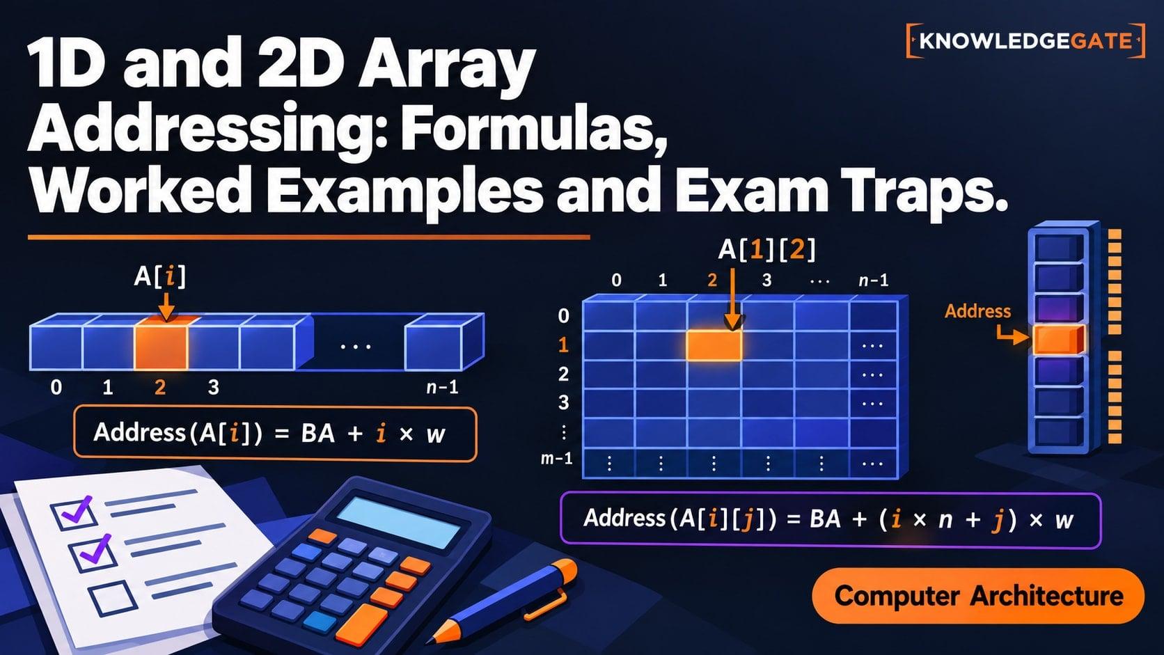
Array-address questions become simple arithmetic after separating four details: the base address, element width, lower bounds and storage order. Mix up one, and a neat calculation can end at the wrong location. Each address follows from the number of complete elements before the target. The row-major and column-major layouts use different multipliers for the same bounded 2D array. Array addressing sits naturally within CS Fundamentals for Exams & Placements, because it connects arrays, indices and memory representation.
What an array address formula is counting
An array stores same-sized elements contiguously. A byte address identifies one byte, while the element width w gives the bytes per element. The declared bounds identify valid indices.
Let B denote the address of the first declared element. For any target, count the complete elements stored between that first element and the target. Multiplying this element offset by w converts it to a byte offset from B.
Every formula follows the same three steps:
Count the complete elements stored before the target. This is the element offset.
Multiply that count by
w. This is the byte offset.Add the byte offset to
B.
C-specific array decay, sizeof behaviour and zero-based row-major arithmetic are covered in Arrays and Strings in C: Decay, sizeof and 2D Addresses. Declared lower bounds require a separate calculation: subtract each lower bound before choosing the row-major or column-major multiplier. Reverse variants then recover an index, base, width or dimension from the address. The CS Fundamentals for Placements by Sanchit Sir course connects the underlying CS ideas.
1D addressing with a non-zero lower bound
For a one-dimensional array A[L..U], first check that L <= k <= U. The number of declared elements before A[k] is k - L, so:
LOC(A[k]) = B + (k - L) * w
The subtraction counts elements; it is not an adjustment to memorise. At k = L, zero elements come before the target, so the formula returns B.
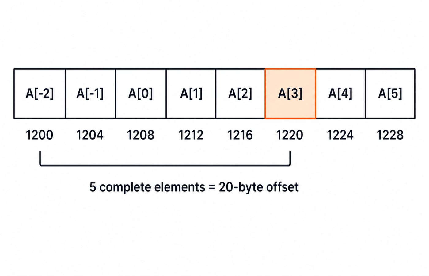
Consider A[-2..5], where B = LOC(A[-2]) = 1200 and w = 4 bytes. To locate A[3]:
Element offset:
3 - (-2) = 5elementsByte offset:
5 * 4 = 20bytesAddress:
1200 + 20 = 1220
Now reverse the process for address 1212. Its distance from the base is 1212 - 1200 = 12 bytes. Dividing by the width gives 12 / 4 = 3 complete elements after the base. Therefore, the index is L + 3 = -2 + 3 = 1, so address 1212 belongs to A[1]. If the byte difference were not divisible by w, the address would not identify an element boundary.
Moving from a 2D grid to linear memory
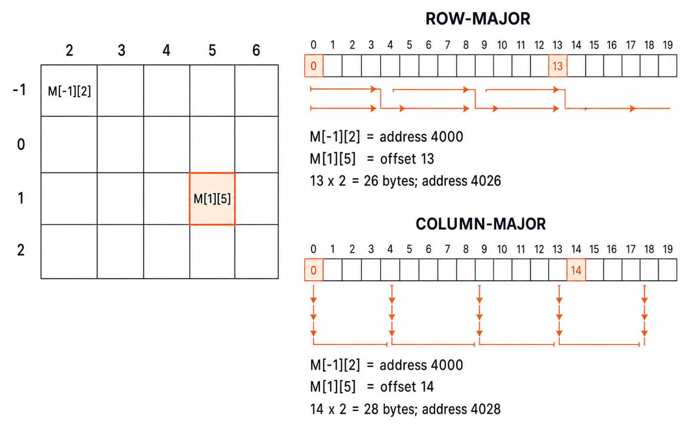
Use one array for both layouts: M[-1..2][2..6]. Its row indices are -1, 0, 1, 2, and its column indices are 2, 3, 4, 5, 6. Therefore:
rows = 2 - (-1) + 1 = 4columns = 6 - 2 + 1 = 5
Let B = LOC(M[-1][2]) = 4000 and w = 2 bytes.
In row-major order, memory finishes all five columns of one row before entering the next row. For target M[i][j], complete rows contribute (i - Lr) * columns, and movement within the target row contributes j - Lc:
LOC(M[i][j]) = B + w * ((i - Lr) * columns + (j - Lc))
In column-major order, memory finishes all four rows of one column before entering the next column:
LOC(M[i][j]) = B + w * ((j - Lc) * rows + (i - Lr))
The declared memory order decides which formula applies; a language convention cannot replace it.
One 2D element in row-major and column-major order
Find LOC(M[1][5]) first in row-major order. Before row 1, the complete rows -1 and 0 are stored. They contain:
(1 - (-1)) * 5 = 2 * 5 = 10 elements
Within row 1, columns 2, 3 and 4 appear before column 5:
5 - 2 = 3 elements
The total element offset is 10 + 3 = 13. The byte offset is 13 * 2 = 26, so:
LOC(M[1][5]) = 4000 + 26 = 4026
Now keep the same target but switch to column-major order. Before column 5, the complete columns 2, 3 and 4 are stored. They contain:
(5 - 2) * 4 = 3 * 4 = 12 elements
Within column 5, rows -1 and 0 appear before row 1:
1 - (-1) = 2 elements
The total element offset is 12 + 2 = 14. The byte offset is 14 * 2 = 28, giving:
LOC(M[1][5]) = 4000 + 28 = 4028
Layout | Full groups before target | Within-group offset | Element offset | Byte offset | Address |
|---|---|---|---|---|---|
Row-major | 10 | 3 | 13 | 26 | 4026 |
Column-major | 12 | 2 | 14 | 28 | 4028 |
There are 4 * 5 = 20 elements and 20 * 2 = 40 bytes in the array. Its element-start addresses therefore run from 4000 to 4000 + (19 * 2) = 4038. Both 4026 and 4028 are aligned to two-byte boundaries and lie inside that range.
Reverse and missing-value variants
For a 1D array, reverse addressing uses:
k = L + (address - B) / w
Confirm that address - B is divisible by w and the recovered index lies within L..U. In the earlier example, (1212 - 1200) / 4 = 3, and -2 + 3 = 1, so the answer is A[1].
For a short 2D variant, take row-major N[1..4][0..5], with B = 800 and w = 4. It has 5 - 0 + 1 = 6 columns. For N[3][4]:
Element offset:
(3 - 1) * 6 + (4 - 0) = 12 + 4 = 16Byte offset:
16 * 4 = 64Address:
800 + 64 = 864
A problem may instead leave B, w, a bound or a dimension unknown. Write the symbolic formula with the declared bounds and layout first, then isolate the unknown. For the N[3][4] example, if the address is 864 but the base is missing, then B = 864 - 4 * ((3 - 1) * 6 + (4 - 0)) = 864 - 64 = 800. Substituting the recovered base into the original formula returns 864, which checks the result.
Exam-style patterns and traps that lose marks
Questions here usually take five forms: calculate an address, recover an index, compare row-major with column-major order, solve for a missing base or dimension, or translate a 2D index into a flattened offset. The practice bank contains more than 40 questions on 1D and 2D Addressing.
Pair every common trap with its correction:
A dimension has
U - L + 1elements, notU - L.Subtract the declared lower bound, even when it is negative or non-zero.
Row-major uses the number of columns as its full-row multiplier.
Column-major uses the number of rows as its full-column multiplier.
Multiply the element offset by
w, never the base address.Keep element offsets separate from byte offsets.
Use the stated layout instead of assuming row-major.
Check bounds before calculating an address.
For a quick scratch routine, write B, w, every lower bound and the layout. Calculate row and column counts. Circle the correct multiplier. Find the element offset, convert it to bytes and add B. Finally, check bounds, alignment and the possible address range. Apply that routine while working through Data Structures MCQs.
The short version and next step
The core memory aid is address = base + element offset * element width. In 1D, the offset is k - L. Row-major counts complete rows and then columns. Column-major counts complete columns and then rows. The formula is short, but accurate counting is the real skill.
Now recompute M[1][5] without looking. Explain aloud why row-major gives 4026 but column-major gives 4028. If the multiplier is hard to explain, return to the grid instead of memorising another formula. For a structured path that places this idea inside sequenced GATE CS preparation, continue with GATE Guidance by Sanchit Sir.
Keep learning

1D and 2D Array Addressing MCQs: 12 Solved Questions
Solve 12 array-address questions step by step, from negative lower bounds and 1D offsets to row-major, column-major, triangular and tri-diagonal storage.
Updated 30 Oct 20268 min readData Structures MCQs

Arrays and Strings in C: Array-to-Pointer Decay, sizeof Traps and 2D Address Arithmetic
Learn what an array name means in C, why sizeof changes across a function boundary, and how to calculate 1D and 2D element addresses without guessing.
Updated 30 Jul 20265 min read164 viewsC Programming & Data Structures
Row Major and Column Major Address Calculation for GATE: 2D Array Numericals Solved
Derive both 2D array address formulas from a flat memory block. The same element is solved in row-major and column-major order for 0-based and 1-based indexing.
Updated 30 Oct 20265 min read304 viewsGATE Strategy & Roadmap

2D Transformations and Algorithms Interview Questions with Worked Answers
Build a convention-first answer to 2D transformation questions, then test it through composite matrices, pivot rotation, polygon code and inverse checks.
Updated 8 Nov 20265 min readInterview Corner